Introduction
In competitive swimming, swimming velocity is determined by the net balance between propulsive and drag forces acting on swimmers to determine the body’s displacement (i.e., accelerations and decelerations, respectively) (Barbosa et al., 2020):
in which a refers to acceleration (m•s-2), T is the total propulsion (N), D is the total drag force (N), and m the swimmer’s body mass (kg). Drag is the resistance force to promote displacement in a fluid environment (such as water), and can be calculated based on Newton’s equation as:
in which D is the drag (N), ρ is the density of water (997 kg•m-3), FSA is the swimmer’s frontal surface area (m2), v is the swimming velocity (m•s-1), and CD is the drag coefficient (dimensionless). There are two types of drag: (1) passive drag, i.e., water resistance over a swimmer being towed through the water without moving body segments, and (2) active drag, i.e., water resistance while swimming (Pendergast et al., 2005). Thus, the latter (i.e., active drag) receives a lot of attention by researchers and coaches since swimmers spend most time of the race performing the swimming stroke (Morais et al., 2019; Veiga and Roig, 2016).
However, the active drag force may not be the most adequate way to understand the hydrodynamic profile of swimmers (the same rational can be used for the passive drag). Drag was found to be proportional to the square of velocity, i.e., an increase in swimming velocity will promote an exponential increase in drag (Toussaint and Beek, 1992). Thus, taking drag as the reference variable for the swimmers’ hydrodynamic profile can lead to misleading assumptions. For instance, when measuring age-group swimmers based on a longitudinal approach, active drag increased significantly (Morais et al., 2014). However, this may not be related to worse swimming technique, but rather to the increase in swimming velocity, which will directly affect active drag (Morais et al., 2014). As it happens in other sports where the fluid resistance plays a key role, such as cycling (Malizia and Blocken, 2021) and motorsports (Katz, 2021), the best way to understand the dynamics of an object is through the drag coefficient. This allows the analysis of the aerodynamic or hydrodynamic effectiveness based on the fluid resistance of an object or subject regardless of its size or velocity.
Besides the drag methods, the active drag coefficient (CDa) can also be calculated through propulsion methods (Havriluk, 2003). Nowadays, there is user-friendly equipment that measure swimmers’ propulsion without any mechanical restrictions (Havriluk et al., 2013; Koga et al., 2020; Lanotte et al., 2018). After obtaining the propulsion generated by the stroke cycle, swimming velocity, and FSA, it is possible to calculate the CDa based on equation (2). However, as far as our understanding goes, evidence on the level of agreement between the CDa measured by drag and propulsion methods is missing. This information is important to understand whether the two types of equipment measure the same phenomenon, i.e., the hydrodynamic profile of the swimmers.
Therefore, the aim of this study was to analyze the agreement of the CDa measurement through drag and propulsion methods. It was hypothesized that there would be a high level of agreement between the different methods of measuring CDa.
Methods
Participants
Eighteen swimmers (nine boys: 15.9 ± 0.9 years, 70.73 ± 9.10 kg of body mass, 1.79 ± 0.07 m of body height, 1.87 ± 0.09 m of the arm span; FINA points: 590.11 ± 61.81 in the 100 m freestyle event, short course meter swimming pool; nine girls: 15.3 ± 1.2 years, 57.64 ± 6.11 kg of body mass, 1.63 ± 0.07 m of body height, 1.67 ± 0.09 m of the arm span, FINA points: 601.56 ± 73.38 in the 100 m freestyle event, short course meter swimming pool) were recruited to participate in this study. Swimmers were recruited from a national squad that included swimmers participating at international championships and national record holders (Tier 3; McKay et al., 2022). They had more than 5 years of competitive experience and performed six to seven swimming sessions per week, complemented with at least one dry-land strength and conditioning training session per week. Parents or guardians and swimmers signed an informed consent form. All procedures were in accordance with the Declaration of Helsinki regarding human research, and the Polytechnic of Bragança Ethics Board approved the research design (N.º 72/2022).
Design and Procedures
The velocity perturbation method was used (Kolmogorov and Duplishcheva, 1992) to compute the active drag coefficient based on a drag method (CDa_VPM). Swimmers performed two 25 m maximum front crawl swimming trials with a push-off start after a standardized warm-up. One trial was performed at maximum speed in front crawl and the other at maximum speed in front crawl while towing a hydrodynamic body (i.e., a perturbation device). This hydrodynamic body was attached to the swimmers’ waist with a belt at an 8 m distance (to minimize drafting effects of the perturbation device in the wake of the swimmer) (Kolmogorov and Duplishcheva, 1992).
In each trial, the string of a speedometer (SpeedRT, ApLab, Rome, Italy) was attached to the swimmers’ hip to measure swimming velocity. The speedometer calculated the displacement and velocity of the swimmer at a sampling rate of 100 Hz. Afterwards, it was imported into signal processing software (AcqKnowledge v. 3.9.0, Biopac Systems, Santa Barbara, USA). The signal was handled with a Butterworth 4th order low-pass filter (cut-off: 5 Hz). A video camera (Sony FDRX3000, Japan) was attached to a rail on the edge of the swimming pool. The camera recorded swimmers in a sagittal plane, and it was synchronized to the speed-time data. Velocity was measured between the 11th and the 24th m as reported elsewhere (Morais et al., 2020a).
The CDa_VPM was computed as:
in which CDa_VPM is the active drag coefficient (dimensionless), Da is the active drag (N), ρ is the density of water (997 kg•m-3), FSA is the swimmer’s cross-sectional frontal surface area (m2), and v is swimming velocity (m•s-1). The FSA was measured by digital photogrammetry. Swimmers were photographed by a digital camera (Alpha 6000, Sony, Tokyo, Japan) in the transverse plane (downwards view) on land simulating the streamlined position. This position is characterized by the arms being fully extended above the head, one hand over the other, fingers also extended close together and head in a neutral position. The FSA was measured from the swimmer’s digital photo on dedicated software (Udruler, AVPSoft, USA) (Morais et al., 2012). Afterwards, a correction was performed based on the FSA variation during the stroke cycle (Morais et al., 2020a).
The propulsion data were acquired concurrently with the drag data (without the perturbation device). As the VPM measured the swimmer’s drag between the 11th and the 24th m, the average propulsion performed during this distance was used for analysis. Force data acquisition equipment Aquanex (Swimming Technology Research, USA) was used to measure the propulsion (f = 100 Hz) (Morais et al., 2020b). This system is based on sensors that estimate the in-water force with a measurement error of 0.2%. Such sensors were placed between the third and fourth metacarpals to measure the pressure differential between the palmar and dorsal surfaces. It is assumed that this place is a good proxy of the application point of the thrust vector on the hand (Gourgoulis et al., 2013). At the beginning of each trial, swimmers were asked to keep their hands vertically immersed at a depth of 0.5 m for 10 s to calibrate the system with the hydrostatic pressure values. The sensors and video output were connected to an A/D converter connected to a laptop on the pool deck with Aquanex software (Aquanex v. 4.2 C1211, Richmond, USA) (Morais et al., 2020b). Afterwards, time-force series were imported into signal processing software (AcqKnowledge v. 3.9.0, Biopac Systems, Santa Barbara, USA). The signal was handled with a Butterworth 4th order low-pass filter (cut-off: 5 Hz).
For each dominant and non-dominant arm-pull, the mean propulsion (Fmean_dominant and Fmean_non-dominant, N) was analyzed. The Ftotal_stroke cycle (the total propulsion produced in one full stroke cycle) was calculated as being the sum of the propulsion produced by the dominant and non-dominant upper limbs. Afterwards, the active drag coefficient based on the propulsive force (CDa_Thrust) was computed by inverse dynamics based on equation (2). In equation (2) D corresponds to the drag force, which can be assumed equal to the average propulsion for constant swimming velocity (Havriluk, 2003). The FSA values were the same as previously used.
Statistical Analysis
The Kolmogorov-Smirnov and the Levene’s tests were used to assess the normality and homocedasticity, respectively. The mean plus one standard deviation, and 95% confidence intervals (95CI) were computed as descriptive statistics. The coefficient of variation (CV, %) was calculated between the CDa_VPM and CDa_pressure sensors.
The intraclass correlation coefficient (ICC) was measured to establish homogeneity through the fraction or proportion of the total variability of the measurements (Koo and Li, 2016). Afterwards, the comparative analysis between methods included: (1) mean data comparison; (2) simple linear regression between values, and (3) Bland Altman plots (Barbosa et al., 2017). For the mean data comparison, the student’s t-test paired samples (p ≤ 0.05), the mean difference with 95% confidence intervals (95CI), and the magnitude of the effect size (Cohen’s d) were computed. This effect size index was interpreted as: (1) trivial if 0 ≤ d < 0.20; (2) small if 0.20 ≤ d < 0.60; (3) moderate if 0.60 ≤ d < 1.20; (4) large if 1.20 ≤ d < 2.00; (5) very large if 2.00 ≤ d < 4.00; (6) nearly perfect if d ≥ 4.00 (Hopkins, 2002).
Simple linear regression models between assessment methods (drag vs. propulsion) were computed. Trendline equation, determination coefficient (R2), standard error of estimation (SEE), 95% of confidence (95CI), and prediction (95PI) intervals were calculated. As a general rule and qualitative interpretation, the relationship was defined as: very weak if R2 < 0.04; weak if 0.04 ≤ R2 < 0.16; moderate if 0.16 ≤ R2 < 0.49; high if 0.49 ≤ R2 0.81, and very high if 0.81 ≤ R2 < 1.0. The Bland Altman analysis included the plot of the mean value of the drag versus the thrust (i.e., propulsion) (Bland and Altman, 1986). A bias of ± 1.96 standard deviation of the difference was adopted as the limit of agreement. For qualitative assessment, it was considered that the analytical modeling data were valid and appropriate if at least 80% of the plots were within the ± 1.96 standard deviation of the difference (95CI).
Results
Table 1 presents descriptive data for males, females and both sexes grouped together (overall). The CV between the CDa_VPM and CDa_pressure sensors was 6.24%. The ICC between the CDa_VPM and CDa_pressure sensors was ICC = 0.928 (95CI: 0.796 to 0.973). Table 2 presents the t-test comparison between methods. The CDa measured with the VPM and with pressure sensors did not present significant differences with a small effect size (Table 2).
Table 1
Descriptive data (mean ± one standard deviation, and 95% confidence intervals – 95CI) for all the variables assessed for males, females, and both sexes plotted together.
[i] FSA – frontal surface area; v – swimming velocity; Da – active drag; CDa_VPM – active drag coefficient based on the velocity perturbation method; Fmean_dominant – mean propulsion of the dominant upper-limb; Fmean_non-dominant – mean propulsion of the non-dominant upper-limb; Ftotal_stroke cycle – total propulsion of the full stroke cycle; CDa_pressure sensors – active drag coefficient based on the pressure sensors.
Table 2
Comparison between the CDa computed based on the velocity perturbation method and on the pressure sensors method (i.e., propulsion).
| T-test comparison | ||||
|---|---|---|---|---|
| Mean difference (95CI) | t-test | p | d [descriptor] | |
| CDa_VPM vs CDa_pressure sensors mensionless | 0.029 −0.002 to 0. | 1.95 | 0.068 | 0.24 [small] |
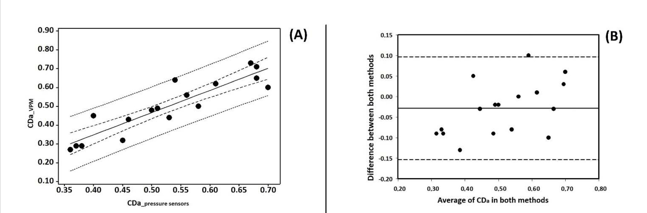
Figure 1 (Panel A) depicts the linear regression (R2 = 0.82, p < 0.001, SEE = 0.06) between methods for the CDa with 95CI and 95PI intervals. The relationship was of very high agreement. Figure 1 (Panel B) depicts the Bland Altman analysis, in which only one swimmer was not within the 95CI agreement. Thus, the agreement criterion, according to which more than 80% of the plots must be within 95CI agreement, was accomplished.
Figure 1
Panel A – linear regression analysis between the active drag coefficient measured with the velocity perturbation method (VPM), and with the pressure sensors. Solid line represents the linear regression trend, dash lines the 95% confidence intervals (95CI), and point lines the 95% prediction intervals (95PI). Panel B – Bland Altman plots of the active drag coefficient measured with the velocity perturbation method (VPM), and with the pressure sensors. CDa_VPM – active drag coefficient based on the velocity perturbation method; CDa_pressure sensors – active drag coefficient based on the pressure sensors.
Discussion
This study aimed to analyze the agreement between measuring the CDa based on drag and propulsion methods. The main results indicate that non-significant differences were observed between the methods with a very high relationship and that the Bland Altman criterion was accomplished.
The literature reports four experimental approaches to measure the active drag: (1) the measuring active drag (MAD) system (Hollander et al., 1986); (2) the assistant towing method (ATM) at constant speed (Alcock and Mason, 2007), and at fluctuating speed (Mason et al., 2011); (3) the residual thrust method (MRT) (Narita et al., 2017), and; (4) the velocity perturbation method (VPM) (Kolmogorov and Duplishcheva, 1992). However, the MAD, ATM, and MRT methods are complex, time-consuming, and expensive systems. On the other hand, the VPM method is simple to set up and therefore less time-consuming, inexpensive, and non-invasive, making it more suitable for the assessment of young swimmers.
Indeed, several studies have used the VPM to measure the hydrodynamics of swimmers (Marinho et al., 2010; Morais et al., 2014; Toussaint et al., 2004) as its reliability to measure the swimmers’ active drag has already been shown (Toussaint et al., 2004). Additionally, most studies related to the assessment of active drag using all three remaining methods (MAD, ATM, and MRT systems) do not present data related to CDa (e.g., Formosa et al., 2012; Hazrati et al., 2016; Neiva et al., 2021). Conversely, studies in which the VPM method was used did present the CDa output (Barbosa et al., 2015; Morais et al., 2014).
Regarding propulsion gear, there are wearable systems that measure the swimmers’ propulsion based on user-friendly setups. These systems are mostly based on independent pressure sensors attached to the swimmers’ hands allowing their displacement such as under “free swimming” conditions (Santos et al., 2022; Koga et al., 2020; Lanotte et al., 2018). A study by van Houwelingen et al. (2017) indicated that research about propulsion must focus on determining the best path and the velocity profile of the hand, hand shape(s) throughout the stroke cycle, and the role of the entire swimmer’s body in producing propulsive force. However, this summary was based on numerical studies. There is no evidence about this topic through experimental procedures and thus, it can be argued that there is still no experimental gold standard method for measuring propulsion in swimming.
Moreover, studies that used this kind of equipment to measure swimmers’ propulsion did not report any CDa output (Koga et al., 2020; Morais et al., 2020b). Nonetheless, it can be argued that the focus of such studies was to mainly understand the swimmers’ propulsion (force that promotes forward motion) and not the water resistance acting on the swimmer’s body. It must be pointed out that the drag MRT method evaluates the drag in front-crawl swimming based on the relationship between propulsion and drag (Narita et al., 2017). It acknowledges that the difference between propulsion and drag occurs from changing the flow velocity, i.e., residual thrust (Narita et al., 2017). In this case, this research group did present the CDa output (Narita et al., 2018a). However, as aforementioned, this method does not rely on an exclusively propulsion method.
Data from the present study showed non-significant differences between the CDa based on both methods and a high level of agreement between them. To the best of our knowledge, this is the only study that aimed to understand the agreement between methods for the CDa measurement, specifically between drag and propulsion methods. Based on the present results, it can be confirmed that the CDa can be measured by different methods as they all measure the same phenomenon. Comparison studies were conducted, but only based on drag procedures and for active drag alone (Formosa et al., 2012; Narita et al., 2018b; Toussaint et al., 2004). However, the overall trend reported in the literature is that the active drag output presents significant differences when measured by different methods. For instance, Toussaint et al. (2004) aimed to compare the MAD and the VPM methods. The authors observed that the two methods produced significant differences in the active drag output, however, they recognized that both methods measured the same phenomenon. Others compared the active drag values between the MAD and the ATM methods (Formosa et al., 2012). For the same mean maximum speed both systems differed by 55% in magnitude and the values obtained were significantly different between the two methods (higher in the ATM). The authors argued that the kicking absence in the MAD system might partially explain such a large difference (Formosa et al., 2012). More recently, Narita et al. (2018b) compared the MAD and the MRT systems without the kicking motion. The active drag values estimated using the MRT method were significantly higher than those obtained by the MAD system. The authors argued that the MAD system implied stroke mechanics constrictions because swimmers must propel themselves by pushing fixed pads underwater (Narita et al., 2018b). Thus, it seems that for this type of measurements, allowing swimmers to move as under “free swimming” conditions represents a key factor.
It must be pointed out that in the present study swimmers used equipment (both drag and propulsion) that allowed them to represent their swimming technique during competition and consequently, their swimming speed. Moreover, it was shown that CDa could be measured by different types of equipment presenting non-significant differences between measurements. In this sense, one can state that researchers, coaches, and swimmers should use the CDa as the main output to evaluate a swimmer’s hydrodynamic profile.
As the main limitations, it can be considered that the propulsion method: (i) relies on a differential pressure system (however, no gold-standard method exists to measure propulsion), and; (ii) measures only the propulsion of the upper limbs. However, one must claim that research has confirmed that the propulsion of the upper limbs accounts for nearly 90% of the swimming velocity (Bartolomeu et al., 2018; Deschodt et al., 1999).
Future studies should rely on: (1) verifying the CDa agreement between other equipment, i.e., drag and/or propulsion, to highlight the CDa as the main hydrodynamic output in swimming, and (2) confirming these assumptions regarding the passive drag coefficient.
Conclusions
It can be concluded that the CDa can be measured through drag and propulsion methods. Non-significant differences with a high level of agreement were found in the CDa measured with both systems. Based on this level of agreement, one can consider that the CDa should be the output taken into consideration to understand the swimmers’ hydrodynamic profile while swimming. Thus, the swimming community is advised to include the CDa whenever assessing active drag in swimming.