Introduction
The search for optimization of sports training processes and, consequently, increased competitive success, has motivated researchers and coaches to deepen their knowledge about the game patterns and flow dynamics, attempting to identify the emergent (Garganta, 2009). In this vein, research centred on match analysis (MA) has proliferated in different sports (Clemente et al., 2015; Melchiorri et al., 2020; Praça et al., 2019; Prieto et al., 2015; Torres-Luque et al., 2020), since it provides detailed in-depth information that has contributed immensely to a better understanding of game dynamics and retrieved implications for the training process (Costa et al., 2012). Sports, especially team sports, evolve either as a dynamic system (Lames and McGarry, 2007; Walter et al., 2007) or a confrontation of dynamic systems (Lebed, 2006). Thus, MA can consider different levels of the systems or even focus only on a specific subset of systems. Although partially independent, these subsystems interact in an interdependent manner, producing diversified behavioural topologies and global organizations (Thelen, 2005; Walter et al., 2007). Consequently, preservation of the ecological sequencing of the game (Mesquita et al., 2013) should be considered at multiple levels (i.e., macro, meso, micro) (Ribeiro et al., 2019).
However, and regardless of the specific methodological approach, research on MA has focused on average performance models (Clemente et al., 2014; Laporta et al., 2015a, 2018a; Sasaki et al., 2017). Despite the tremendous contributions from studies such as these, the more comprehensive look at the different performance models will depend on the research question, in which a whole-sport approach or a single-team approach has different purposes and is complementary. Although research on expertise has been highlighting the coexistence of multiple paths towards expert performance (Ackerman, 2014; Burgess and Naughton, 2010; Vaeyens et al., 2008), some studies have attempted to understand the specific performance paths and characteristics (Buldu et al., 2019; Sarmento et al., 2020). In addition, in the future, it would also be important to analyse each player separately, since within a team each player may have very specific behaviours (Castañer et al., 2016; Maneiro Dios and Amatria Jiménez, 2018). The acknowledgement of a plurality of pathways to expert performance should lead to examine the diversity of performance models at the highest levels of practice. For example, despite height being a major factor in high-level volleyball (Martín-Matillas et al., 2014; Sheppard et al., 2011), elite women’s volleyball has a few national teams of short average stature, such as Japan and Thailand (Vargas et al., 2018). Distinct morphophysiological profiles interact with diversified sociocultural constraints (Grasgruber et al., 2014), resulting in a plethora of developmental relationships that should be explored.
In this context, social network analysis (SNA) emerges as a tool that provides a systemic overview of game patterns (Wäsche et al., 2017), affording an analysis of the dynamic and complex nature of any sports game (Passos et al., 2011). Through a mapping of connections between and within subsystems (McGarry et al., 2002; Walter et al., 2007), SNA allows the creation of networks that expose relationships (edges) between variables of interest (nodes) (Boulding, 1956). The application of centrality metrics provides a measure of the influence of each node within a given network (Lusher et al., 2010; Opsahl et al., 2010; Tsvetovat and Kouznetsov, 2011). Obviously, SNA is a tool, and thus it can be used differently, depending on the purposes motivating a given research piece.
Several interesting studies have applied SNA in different sports (Clemente et al., 2015; Dey et al., 2017; Praça et al., 2019) and to answer different problems (Fewell et al., 2012; Ribeiro et al., 2019; Sasaki et al., 2017). In recent years, our research team has applied SNA to high-level volleyball (Hurst et al., 2016; Laporta et al., 2018a, 2018b, 2019; Loureiro et al., 2017). For example, Hurst et al. (2016) and Loureiro et al. (2017) analysed the interaction of game actions belonging to side-out, side-out transition and transition (KI, KII and KIII) using eigenvector centrality, while Hurst et al. (2017) used similar methodology to analyse attack coverage and freeball (KIV and KV). More recently, Laporta et al. (2018a, 2018b) analysed all game complexes in an interconnected manner and weighting both direct and indirect connections. This body of research has provided proof of concept of the usefulness of SNA when applied to understand game dynamics in volleyball, as well as delivered relevant information such as the predominance of off-system playing (i.e., most setting and attacking actions occur under non-ideal conditions). Laporta et al. (2019) went a step further and attempted to understand if different networks could be associated and would present differences in efficacy levels in the six existing game complexes in high-level men’s volleyball.
Overall, MA affords the identification of regularities that provide greater understanding of the game dynamics. Despite these advances, the above-mentioned research aggregated data from different teams into a single, generalized model. This practice may mask significant differences in the game models and, consequently, in the performance models of distinct teams. Such a data view is likely to provide a monotonic account of a plural phenomenon (Vargas et al., 2018). Inter and intraindividual variability in development and in response to training stimuli is a well-recognized reality (Bompa and Buzzichelli, 2018). We contend this framework should be expanded for encompassing team performance as well. Therefore, the purpose of this study was to understand to what extent different game models can coexist at the highest levels of performance. We applied this rationale to high-level women’s volleyball, and although the sample was from 2014, our aim was to provide proof of concept and pave the way for alternative approaches to MA.
Methods
Sample
The World Grand Prix was one of the major women’s volleyball competitions and has recently been renamed the Volleyball Nations League. Held annually, the competitive format included several stages, after which the six best teams would advance to the finals. Here, the six national teams participating in the finals were analysed (Brazil was 1st in the competition and 4th in the 2014 world ranking; Japan was 2nd and 6th, respectively; Russia was 3rd and 5th; Turkey was 4th and 12th; China was 5th and 1st; Belgium was 6th and 16th). The entire matches played by these teams in the finals were analysed (n = 15 matches, 56 sets, 7,176 ball possessions).
Design and Procedures
The matches were obtained from laola.tv (public domain matches) and viewed in a highdefinition format (1080 p). The perspective was lateral (i.e., aligned with the net and with a moving camera). Variables were defined in accordance with the possibilities afforded by this type of a recording. Data were registered in a worksheet generated in Microsoft® Excel® 2017 for Mac (Version 15.30, USA) and later analysed using IBM® SPSS® Statistics for Mac (Version 24, USA) for controlling data quality (i.e., verifying incorrect codes, cataloguing mistakes, etc.). Initial analysis was conducted by an observer who was alevel III volleyball coach, with a master's degree and more than 10 years of experience in the field. For the purpose of assessing reliability of the observations, we randomly selected 18.6% of the actions (n = 1,335 plays). Interobserver reliability was conducted by a high-level volleyball coach that did not belong to the research team. Intraobserver reliability was verified one month after the original observations and Cohen’s Kappa ranged from 0.803 to 0.980 (Table 1), which is above the 0.75 cut value proposed by Tabachnick and Fidell (2007).
Table 1
Kappa values and standard error for all variables.
Measures
The Serve Type was adapted from Costa et al. (2012) and included three categories: power jump serve (PJS), floating jump serve (FJS) and standing serve (SS). The Serve Trajectory combined where the server was serving from (i.e., behind the line in zones 1, 6 or 5) (Quiroga et al., 2010) and six target zones (García-Tormo et al., 2006), corresponding to the official zones of the court. For example, the code 16 means the server was behind zone 1 and the reception occurred in zone 6. Since preliminary data analysis revealed a very reduced frequency of occurrence of short serves to zones 2, 3 and 4, these three categories were grouped into a single category denoting the short serve (s).
The Setting Row denoted whether the setter was playing in the defence zone (DZ) (i.e., zones 1, 5 or 6) or in the attack zone (AZ) (i.e., zones 2, 3 or 4), as defined by the international rules of the Fédération Internationale de Volleyball (FIVB; available at http://www.fivb.org/EN/Refereeing-Rules/RulesOfTheGame_VB.asp).
The Setting Conditions indicate the amount and the type of setting options, i.e., the attack options that the setter can potentially use. This variable was defined according to Laporta et al. (2018a), i.e., under setting condition A (SCA), the setter has all attack options available; under setting condition B (SCB), the setter can still use quick tempos, but some attack options are not available (e.g., attack combinations involving the crossing of players); under setting condition C (SCC), the setter can only deploy slow attack tempos in the extremities of the net or in the backrow. The Attack Zone comprised the six official volleyball zones stipulated by the FIVB rules, and numbered from 1 to 6. Attack Tempo refers to the timing of the attack, and is therefore a relative measure. Four categories were defined, adapted from Afonso et al. (2010): in tempo 1 (T1), the attacker jumps in close proximity with the setting action; in quick tempo 2 (T2Q), the attacker uses two foot actions after the setting; in slow tempo 2 (T2S), the attacker uses three foot actions after the setting; in tempo 3 (T3), the attacker uses more than 3 foot actions after the setting or uses 3 foot actions but only starts after a brief waiting compass.
Attack Combinations were defined according to Vargas et al. (2018) as the intentional collaboration of different attackers through manipulation of attack zones and/or tempos. Three different types of combination were considered: simple play (SP), in which the middleattacker uses tempo 1 and the remaining attackers attack tempos 2 or 3 in their base positions; zone overload (ZO), where the middle-player uses tempo 1 and another attacker closes-in the middle-player space to attack a tempo 1 or 2; and crossings (CP), where an attacker crosses behind another to attack in a different zone. Even if the players participating in a given combination were not solicited (i.e., the setter would set the ball to a player not involved in the combination), the play would be registered, since it likely induces effects on the opposing block.
Attack Efficacy followed the proposal of Palao and Ahrabi-Fard (2011), having considered five categories: attack error (A0); attack that affords the opponent a counter-attack with all the attack options (A1); attack that affords the opponent good conditions for the counter-attack, but inhibiting some attack combinations and making it difficult to use tempo 1 with the middle-attack (A2); the opponent struggles to counter-attack and can only use high balls or return a freeball (A3); the attack scores a point (A4). Block Opposition was adapted from Afonso and Mesquita (2011) and had five categories: no blocking (B0); single blocking (B1); double blocking (B2); broken double blocking (B2B); and triple blocking (B3). The Number of Defensive Lines reported on the number of imaginary lines parallel to the net formed by players when defending (Laporta et al., 2015a, 2015b). The number of defensive lines was also registered for attack coverage (KIV).
Statistical Analysis
Finally, SNA with calculation of degree centrality was performed using Gephi© 0.9.1 for Mac (Version 10.10.3, France). While SNA allows calculating interactions between nodes (Passos et al., 2011; Tsvetovat and Kouznetsov, 2011) and understanding their relative importance in a global context (Lusher et al., 2010; Morales et al., 2008), degree centrality provides a measure of the power or influence of a node within a network considering the sum of all direct connections from one node to another (Lusher et al., 2010; Opsahl et al., 2010; Tsvetovat and Kouznetsov, 2011). Here, although only considering the direct connections between the nodes through non-weighted and undirected digraphs (Wasserman, 1994), the sum of the number of connections of a node was considered using the formula: DC = deg(n)/n-1, where deg(n) corresponds to the number of connections of a node, divided by the total of nodes minus 1 (Freeman, 1979). This centrality measure was used to show in a crude way the main differences between the national teams. The game actions in volleyball present a sequence in each ball possession, thus each connection was considered when an influential game action in the next one occurred, for example, the first game action was a serve (presenting the categories: serve type and serve trajectory), which then linked to the construction of the attack from the reception (setting row, setting conditions, attack zone, attack tempo, attack combination and attack efficacy), and later yet proceeded to variables related to defence (block opposition, number of defensive lines) and counterattack (same attack variables mentioned above). In this sense, a rally can have different sequences and ending points, such as a jump float (serve type) - serve trajectory 15, attack zone (setting row) - setting condition A - attack zone 3 - attack temp 1 - simple play - attack efficacy 0. After this step, the data were presented separately for each national team, along with the range of values between all of them with the minimum and maximum value for each variable. For example, a power jump serve with inter-team variation, with degree centrality ranging from 0 (the Japanese team did not perform any serve of this type) to 27 (Chinese team with the highest value).
Results
Social network analysis with degree centrality was used to create the networks for the six different national teams (Figures 1 to 3). China presented the highest number of connections (26,826), followed by Russia (22,739), Turkey (22,391), Brazil (22,130), Japan (20,826) and, lastly, Belgium (20,087).
Figure 1
Networks of Brazil and Japan teams with the measure of degree centrality.
Legend: PSJ - power jump serve; FJS - floating jump serve; SS - standing serve; 11, 15, 16, 61, 65, 56, 51, 55, 56, ST- serve trajectory; SRAZ - setter in the attack zone; SRZD - setter in the defensive zone; SC A to C- Setting Condition A to C; AZ1 to AZ6 - attack zones 1 to 6; AT1, AT2R, AT2L, AT3 - attack tempo 1 to 3; SP - simple play; ZO - overloaded zone; C- crossings; A0 to A4 - attack efficacy; B0 to B3 – block opposition with zero to three blockers; LD1 to LD3 - one to three defensive lines.
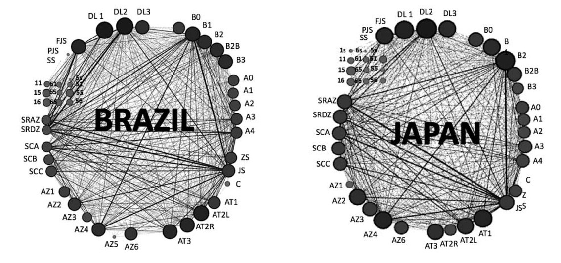
Figure 2
Networks of Brazil and Japan teams with the measure of Degree Centrality.
Legend: PSJ - power jump serve; FJS - floating jump serve; SS - standing serve; 11, 15, 16, 61, 65, 56, 51, 55, 56, ST- serve trajectory; SRAZ - setter in the attack zone; SRZD - setter in the defensive zone; SC A to C- Setting Condition A to C; AZ1 to AZ6 - attack zones 1 to 6; AT1, AT2R, AT2L, AT3 - attack tempo 1 to 3; SP - simple play; ZO - overloaded zone; C- crossings; A0 to A4 - attack efficacy; B0 to B3 – block opposition with zero to three blockers; LD1 to LD3 - one to three defensive lines.
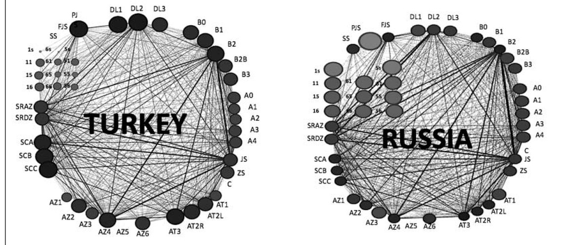
Figure 3
Networks of Brazil and Japan teams with the measure of Degree Centrality.
Legend: PSJ - power jump serve; FJS - floating jump serve; SS - standing serve; 11, 15, 16, 61, 65, 56, 51, 55, 56, ST- serve trajectory; SRAZ - setter in the attack zone; SRZD - setter in the defensive zone; SC A to C- Setting Condition A to C; AZ1 to AZ6 - attack zones 1 to 6; AT1, AT2R, AT2L, AT3 - attack tempo 1 to 3; SP - simple play; ZO - overloaded zone; C- crossings; A0 to A4 - attack efficacy; B0 to B3 – block opposition with zero to three blockers; LD1 to LD3 - one to three defensive lines.
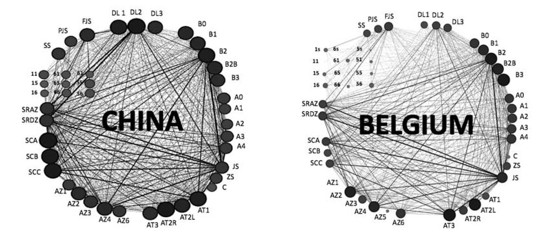
While Figures 1 to 3 present the overall network and afford qualitative interpretation, Tables 2 and 3 presents the quantitative values for degree centrality. The range column provides the minimum and maximum observed centrality values for each variable. While there were differences in the serve trajectory, it was in the serve type where the networks showed more expressive differences in gameplay. The power jump serve was almost not used by three teams (Turkey, Russia and Japan), one team using it occasionally (Brazil), and two teams using it considerably (Belgium and China). On the other end of the spectrum, the standing serve was negligible in three teams (Brazil, Turkey and Japan), while frequently used by Russia, Belgium and China. Of note, while most teams showed a strong centrality value focused on just one type of a serve (e.g., Brazil, Turkey and Japan committing to the float jump serve), Russia’s centrality values denoted a balance between the float jump serve and standing serve, while Belgium and China had balanced centrality values across all three categories.
Table 2
Degree Centrality (frequency of occurrence) for the variables.
Table 3
Degree Centrality (frequency of occurrence) for the variables.
[i] Legend: Setting row: AZ – Attack zone, DZ – Defence zones; SC A, B and C- Setting condition A, B and C. AT1 - Attack tempo 1, AT2Q – Attack tempo 2 quick, AT2S – Attack tempo 2 slow, AT3 - Attack tempo 3; SP - Simple play, ZO - Zone overloaded, CP – Crossing play; AE0, 1, 2, 3 and 4 - Attack efficacy 0, 1, 2, 3 and 4. B0 - No block, B1 - Simple block, B2 - Double block, B2Q - Broken double block, B3 - Triple block.
Setting row presented a balanced participation for all teams between the defensive zone and the offensive zone. Setting conditions presented a balanced centrality distribution between ideal, close to ideal and non-ideal conditions (i.e., A, B and C) for all teams, with the exception of China, which presented predominance of good setting conditions (i.e., A and B). The attack zone showed major differences between the competing teams. Belgium and Japan presented the lowest values for attacks in the extremities of the net, while Russia and China had the highest values. Solicitation of the middleattacker also revealed major differences in gameplay, on the lower end were Brazil and Russia, while China was on the upper end. Attack tempo also allowed distinguishing between the teams. Tempo 1 had a centrality range of 20 to 33 (Belgium and China, respectively), and tempo 2 showed a range of 24 (Belgium) to 35 (Russia and China). Tempos 2 quick and 3 were more wellbalanced and had fewer inter-team variation. As for attack combinations, simple plays and zone overload presented balanced values for all teams, with the exception of Belgium, with much greater centrality for simple play than zone overload. Attack efficacy was balanced across conditions and teams.
As for the block opposition, teams presented a balanced distribution of centrality values across all categories, with few exceptions. The range of values for triple blocking was greater than for the other categories, therefore having a greater interteam variation. In this regard, Japan was an outlier, having the lowest centrality values for noblocking and triple blocking, which may relate to strategic options in positioning the block. The number of defensive lines also presented considerable variations.
Discussion
Performance analysis has provided powerful contributions to the knowledge of game dynamics and useful information for improving training processes (Garganta, 2009; Hughes and Bartlett, 2002). Notwithstanding, studies using MA have focused on average models, and our previous studies are not exception (Hurst et al., 2017; Laporta et al., 2018a, 2019). These studies are important to understand what leads teams to win matches. However, using an approach which focuses on specific characteristics which are different and complementary, also leads to sporting success. Here, the goal was to understand to what extent game models could vary within the highest level of performance in women’s volleyball. We re-analysed data from the 2014 World Grand Prix, and our aim was to provide a proof of concept with regard to the importance of considering the plurality of performance models and the dangers of focusing on a single, averaged-out model. The main message is more relevant than the specific results.
Here, however, we attempted a paradigm change and adopted an approach that would respect the idiosyncrasies of each competing team, thus creating a model for each team instead of an aggregate model using a set of tools of social network analysis. We are convinced that exposing how different high-level teams can be effective using distinct approaches to the game will provide coaches with a wider understanding of the possibilities of achieving success, and also invite coaches to explore their own team skills instead of copying a standardized model, also because the characteristics of individual players may vary drastically at elite levels (Vargas et al., 2018).
First and foremost, the six networks shown in Figures 1 to 3 demonstrate differences in game patterns, with different teams having diversified distributions of their centrality values. This is even more important as volleyball is a sport where game sequences do not afford as much variability as other team sports, because of the rules inhibiting the prehension of the ball and limiting the number of contacts per ball possession. The visual differences are confirmed by the quantitative values presented in Table 1. As apparent from the analysis of the table, ranges of degree centrality values are extensive and illustrate how game patterns differ significantly between the networks, i.e., between the different teams. This occurred despite the matches between the six teams all belonged to the finals of a major world competition.
The serve type, for example, showed significant differences between the six national teams. Whereas Belgium and China made consistent use of the power jump serve, other teams almost did not use this type of a serve. The standing serve was commonly used by Russia, Belgium and China, but not by the other three teams. These data are in accordance with the literature, in which, although the jump serves do not appear frequently, the standing serves are still important part of women's volleyball (Hurst et al., 2016; Palao et al., 2009). This means very different implications for the opposing reception strategies. Major differences were also observed for attack zones and tempos. For example, tempo 1 was more central in the game patterns of China than those of Russia and Brazil, despite the fact that all three teams were elite competitors. There were also additional differences. However, we should again point out that the goal was to establish the need to study the differences between teams, instead of aggregating data into an idealized model (Hughes and Bartlett, 2002), even because top-level volleyball teams have been reported to vary considerably in anthropometric data (Vargas et al., 2018).
Interestingly, the different game patterns did not seem to interfere with attack efficacy. Even though a few studies in volleyball have suggested that game patterns correlate with different efficacy levels in the attack (Marcelino et al., 2008; Mesquita et al., 2013; Silva, Marcelino et al., 2016), others have shown differently, and have gone as far as suggesting that the individual skill of the attacker may be more relevant for the result of the attack action than the game patterns preceding it (Afonso and Mesquita, 2011; Laporta et al., 2019). This may be related to the fact that blockers cannot actively try to steal the ball away from the attackers; instead, they are forced to wait for the attacker to touch the ball, which provides an edge to the attacker.
Beyond support for the need to carefully analyse the inter-team variability with regard to game patterns, our data further suggest that, if different approaches to the game are coexisting at the highest levels of performance, then perhaps talent identification processes should also respect the existence of multiple profiles and multiple paths towards expertise (Ackerman, 2014; Vargas et al., 2018). This does not detract from the relevance of height as a major factor for success in volleyball (Sheppard et al., 2011), but there are well-recognized exceptions at the highest levels of performance (Vargas et al., 2018).
Practical Implications
We provided an account of inter-team variability in game patterns at the highest levels of performance of women’s volleyball, but we believe this framework could be expanded to men’s volleyball and, especially, to successful youth teams. Furthermore, even in the context of team sports, individual performances may produce a strong impact on global performance and, especially, change a team’s dynamics (Silva, Sattler et al., 2016). Different approaches to play will provide coaches with an expanded understanding of individual and collective possibilities for achieving success, rather than copying team models with different characteristics from their context.
Limitation and Future Studies
Despite eigenvector centrality being more robust and showing even more nuanced connections between the variables (since it also weights indirect connections), here, we used the simpler degree centrality as a test-case to try to understand whether a simple metric could afford an identification of the main differences in game patterns between national teams. This was indeed possible, even in a sport (i.e., volleyball) where game sequences are more predictable and determinist than other team sports (due to the prohibition of grabbing the ball and also due to the limitation of the number of contacts in each ball possession). In addition, although we intended to broaden the look given to the analysis of the game, we focused on the inter-team differences in game patterns, thus we chose to use a simpler methodology to check whether our theoretical point would be sufficient to highlight such features. Moreover, if simple, easy to use and calculate metrics are good enough for a given theoretical problem, more complex metrics may not be warranted or at least not strictly necessary.
Notwithstanding, future studies could benefit from using and comparing different metrics (e.g., comparing degree centrality with eigenvector centrality), to better assess to what extent they provide more refined and/or different types of information. Moreover, as all centrality metrics are influenced by the absolute number of connections, perhaps it would be advisable to start analysing these metrics using standardized scores. Thus, the effect of teams having played different amounts of sets and/or points or having played rallies with different duration could perhaps be accounted for.
Conclusions
In conclusion, this study shows that even at the elite level, different teams can present different regularities or patterns of play. Thus, when considering the individual characteristics and skills of each team, coaches can create different and more effective game models, instead of mirroring game models of other teams with characteristics different from their context.