Introduction
Research into the ability to maintain body balance are among the basic measurements performed both in sports training as well as during the diagnosis of many different diseases, in particular neurological diseases. Among the measurements taken, the tests are dominated by standing still and differentiated for measuring eyes open and closed. The process of maintaining balance is, however, a very complex process in which many systems are involved, both at the level of collecting information from the outside world as well as at the central nervous system level. Therefore, measurements under static conditions may be insufficient and measurements under dynamic conditions may be more necessary. Examples of such measurements include those in which the tested person is to perform specific motor tasks, maintain balance on an unstable (Creath et al., 2005) or moving ground and/or platform (Maurer et al., 2003; Wiszomirska et al., 2017) or stand still in a moving environment (Lestienne et al., 1977; Maurer et al., 2003; Jurkojć et al., 2017). These types of measurements, which differentiate the stimuli perceived by the individual senses that help maintain balance, are known as tests in sensory conflict conditions. One of the ways of conducting this type of test enabling the determination of the impact of the sight organ on maintaining balance is to simulate the movements of the environment with the examined person standing on stationary ground. Such tests have proven that visual disturbances significantly affect the ability to maintain balance and a moving environment reduces human stability (Lestienne et al., 1977; Sundermier et al., 1996; Juras et al., 2019).
The use of computer techniques has significantly facilitated research with moving scenery, enabling a greater variety of presented images. Such research has been conducted, among others, by Alahmari (Alahmari et al., 2014), Cleworth (Cleworth et al., 2016), Robert (Robert et al., 2016), Tossavainen (Tossavainen et al., 2003) and Horlings (Horlings et al., 2009), who, together with their teams assessed the impact of created scenery on maintaining body balance, demonstrating the obvious impact of virtual reality on reducing the stability of the body. Similar studies presenting some relationships between the parameters of moving scenery and maintaining balance were conducted by the team of Keshner (E. A. Keshner et al., 2004; E. Keshner et al., 2004; Streepey et al., 2007), Cunningham (Cunningham et al., 2006) as well as Jurkojć, Michnik and Wodarski (Jurkojć et al., 2017; Jurkojć, 2018; Wodarski et al., 2019).
With new measurement techniques being used more and more often when testing the ability to maintain body balance, there are almost no new methods for analyzing the obtained results which are implemented practical application. The analysis of the human body’s ability to maintain balance based on measuring subsequent COP (Center of Pressure) positions is still one of the basic diagnostic methods of problems with balance used in medical facilities (Scoppa et al., 2013; Polechoński et al., 2016; Brachman et al., 2017). It is assumed that increases in the values of measured parameters, such as the path length of COP or the ellipse area, correlates with problems occurring with balance (Hue et al., 2007; Kocjan et al., 2018); however, such measurements may not be enough (Błaszczyk et al., 2003) and evidence may be found that such relationships do not exist in every case (Sundermier et al., 1996). What is more, if the analysis of results carried out in the standard way was justified in tests for subjects standing still with their eyes open and closed, the use of a moving environment completely changes the behavior of the examined subjects. The conducted research indicates that a moving environment causes, both for healthy and unhealthy people, additional body movements that increase the values of standardly analyzed quantities (Lestienne et al., 1977; Jurkojć et al., 2017).
This fact makes standard analyses based on these quantities very problematic. It can be quite difficult, or even impossible, to assess what increase in the analyzed values should be treated as a symptom of problems with balance. It may turn out that there are no values which can be treated as limits determining the correct and incorrect method of balance. Therefore, other methods of analyzing results should be used for this kind of test. In addition, the lack of advanced methods to analyze the results of measurements of the ability to maintain balance in conditions of sensory conflict means that a lot of valuable information is not evaluated. This appears to be particularly important in view of the fact that virtual reality technology is increasingly used both in sports training and medical applications.
The main goal of the research was to indicate the possibility of supplementing traditional methods of measuring the ability to maintain balance, based on analyzes conducted in the time domain, with other methods which include frequency analysis. The aim of the work was to develop a methodology for the practical use of frequency-domain analyses to quantify the ability to maintain body balance during measurements using a moving environment. It was shown that the results obtained in the frequency domain can complement the results determined in the time domain and how to interpret them. In addition, an analysis of how different parameters of moving scenery influence the ability to maintain body balance are presented.
Using analyzes conducted in the frequency domain, body movements can be divided into at least two types: movements performed at the frequency of the moving environment and movements performed at other frequencies (Jurkojć, 2018). The amplitudes and frequencies of these movements as well as changes in time may indicate problems with maintaining one’s balance.
Methods
Research group
A group of 27 healthy volunteers (13 women and 14 men) took part in the study. The average height was 1.71 m and the weight 64 kg (BMI for each participant did not exceed 30). The average age of participants was 22.4 years.
This study was previously approved by the Ethics in Research Committee of the Academy of Physical Education in Katowice (protocol number 11/2015).
Measuring sequence
6 trials were conducted by each participant. Two of them were conducted in a real environment (eyes open – EO, and eyes closed – EC), and the next four in a virtual environment. Each measurement lasted 50 seconds. Before the measurement, each participant was informed about the study and was able to familiarize him/herself with the virtual scenery. Then, the subject had to stand barefoot, motionless on the measuring platform in an upright position, with feet set at hip-width apart and arms crossed at the chest, focusing on a point located in front of subject at sight level.
During measurement in the virtual environment, the presented scenery oscillated in sagittal plane. The oscillations started at 10 seconds and lasted 30 seconds. COP positions were recorded during the whole trial of 50 seconds.
The oscillations took place with a constant frequency 0.7 Hz or 1.4 Hz, or changed in the middle of the measurement between those two. The selection of the plane of motion as well as frequencies were done on the basis of results from previous research, where these parameters caused bigger disturbances compared to lower frequencies.
Measurement methodology
All measurements of COP positions were conducted on the Zebris FDM-S platform. Virtual sceneries were presented using the Oculus DK2 system. The scenery was created in the Unity 3D engine and was designed as a furnished room or view of a desert.
In measurements in which the scenery was in motion, the following assumptions were made for this movement:
The basic, oscillatory movement of the scenery took place in the sagittal plane of the examined subject (Y axis) according to equation 1:
where:
ft – frequency of scenery motion [Hz],
Ay – amplitude of scenery motion [cm],
t– time [s];
An additional movement increasing the subjective sense of the realism of the moving environment was a rotation around the transverse axis of the body according to equation 2:
where:
fr – frequency of scenery motion [Hz],
Aφ - amplitude of scenery motion [deg],
t– time [s].
The following values of the parameters were assumed: Ay = 15 [cm], Aφ = 1 [deg], fr = 0.5∙ft [Hz]. Translation frequency was equal to ft = 0.7 [Hz] and ft = 1.4 [Hz] – depending on the measurement trial.
Use of the Balance Disturbances Coefficient and Sensitivity Coefficient to assess the influence of moving scenery on subjects
The Short-time Fourier transform STFT was used to analyze changes in the impact of moving scenery over time on maintaining balance by the subjects. The following parameters were adopted:
To conduct the analysis in a quantitative manner, two coefficients were used: the Balance Disturbances Coefficient and Sensitivity Coefficient. The Balance Disturbances Coefficient is a value determined on the basis of the FFT graph obtained for subsequent COP positions. Its value depends on the number of cyclic components appearing, the amplitude values of these components and the frequency corresponding to them. It is determined by applying formula 3:
where:
D– Balance Disturbances Coefficient,
An – amplitude value of the nth cyclic component (maxima on the FFT chart), assuming that the value of the amplitude must be greater than 0.5, fn – value of frequency of the nth cyclic component, N– total number of cyclic components detected.
The calculation of the coefficient value did not take into account the component appearing at the frequency equal to the frequency of scenery movements. This approach eliminated the component of COP motion corresponding to the motion of a body following the scenery. It also allowed the determination of the “amount” of movement with different frequencies, which in effect made it possible to determine how much the person was off balance. A detailed procedure for calculating the coefficient is presented in the paper by Jurkojć (2018).
In order to isolate and assess the subject’s movement of following this scenery, the Sensitivity Coefficient was determined as square of the amplitude value of the cyclic component appearing at the frequency equal to the frequency of scenery movement (0.7 Hz or 1.4 Hz).
The calculation of the values of both coefficients based on STFT charts for each moment of time allowed the determination of changes in the value of these coefficients over time. Examples of charts obtained on the basis of the described methodology are presented in figure 1.
Figure 1
An example of results obtained for a selected person for a measurement performed with a scenery oscillated with a frequency 0.7 Hz in the first 15 seconds and 1.4 Hz in the second 15 seconds (time with disturbance between 15 and 45 second). a) Sensitivity Coefficient S, b) Balance Disturbances Coefficient D. Solid line – the beginning and the end of the scenery movement, dashed line – change in the frequency of the scenery movement
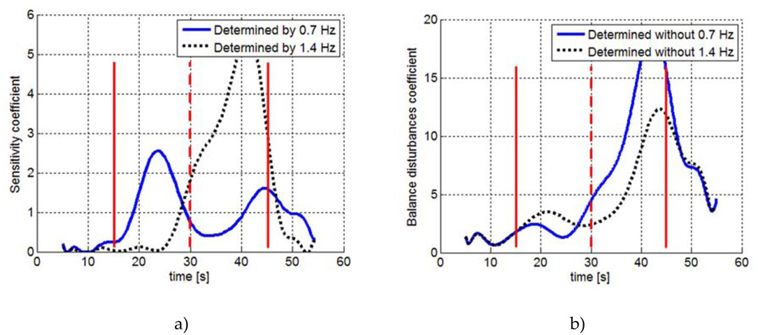
The analysis of both coefficients enabled the simultaneous assessment of general unbalance under the influence of moving scenery (Balance Disturbances Coefficient) and the susceptibility of the subjects to the movements of the scenery manifested in the movement following the scenery (Sensitivity Coefficient).
Description of the methodology for analyzing test results
30-second intervals were separated for the obtained time courses of subsequent COP positions. In the case of measurements with virtual disturbances, this involved the time when these disturbances occurred, while in the case of measurements with eyes open and closed the middle time interval of the measurement was used. Then, each 30-second interval defined in this way was divided into two smaller intervals:
For measurements with a frequency change, the end of the first interval was also a moment of time when the oscillation frequency of the scenery changed. The division into two periods of time was meant to enable the determination of how the impact of virtual disturbances changes over time.
For each of the periods of time and for each of the subjects, the following parameters were determined:
mean COP velocity towards the AP direction,
the area under the curve of the Balance Disturbances Coefficient and the Sensitivity Coefficient.
The area calculations were carried out as follows:
when the scenery was moving at a frequency of 0.7 Hz, the area was calculated under the Balance Disturbances Coefficient curve obtained without the cyclical component at 0.7 Hz and under the Sensitivity Coefficient curve obtained for 0.7 Hz,
when the scenery was moving at a frequency of 1.4 Hz, the surface area was calculated under the Balance Disturbances Coefficient curve obtained without the cyclical component occurring at 1.4 Hz and under the Sensitivity Coefficient curve obtained for 1.4 Hz.
Subsequently, for each parameter determined for all participants, the median, lower and upper quartile as well as the maximum and minimum values were calculated. Tests of the significance of statistical differences were carried out using the Wilcoxon paired order test assumed the significance limit p = 0.05. The MATLAB environment program and the STATISTICA 13 program were used for these calculations.
In addition, to make it possible to indicate the number of people who had an increase or decrease in values of the analyzed quantities between the first and second half of the measurement, the difference between each parameter obtained in the second half and in the first half of the measurement was calculated. In the case of areas under the coefficient curves, the differences were calculated according to the scheme presented in Table 1. Different numbers of measurements occurring for individual measurements resulted from the necessity of rejecting the results classified as thick errors.
Table 1
The method of calculating the differences between the parameters obtained in the first and second half of the measurement. The symbols S0.7 and S1.4 denote the values of the Sensitivity Coefficient determined for the frequencies of 0.7 Hz and 1.4 Hz, respectively, while the symbols D0.7 and D1.4 indicate the values of the Balance Disturbances Coefficient determined without the cyclic component appearing at the frequencies of 0.7 Hz and 1.4 Hz, respectively. The numbers 0-15 and 15-30 indicate the first and second half of the measurement.
Results
Analysis of the results obtained for the whole group
The graphs in figure 2 and 3 show the medians of the mean COP velocities and areas under the coefficients’ courses obtained for all types of measurements.
Figure 2
Medians of the mean COP velocity V in the AP direction, lower and upper quartile and maximum and minimum values
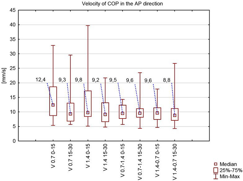
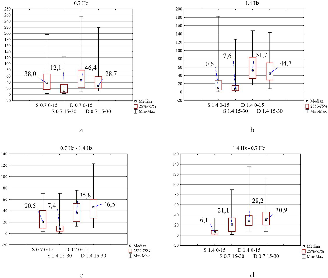
Figure 3
Medians of the areas under the curve, lower and upper quartile and maximum and minimum values. Measurements with a frequency of scenery oscillations equal to: a) 0.7 Hz, b) 1.4 Hz, c) changing frequency from 0.7 Hz to 1.4 Hz, d) changing frequency from 1.4 Hz to 0.7 Hz. S – Sensitivity Coefficient, D – Balance Disturbances Coefficient
Analysis of the medians of mean COP velocities in the AP direction (fig. 2) show that statistically significant differences occurred between the results of tests performed at a constant frequency of 0.7 Hz (p = 0.007) as well as 1.4 Hz (p < 0.001). For both frequencies, the medians of the mean COP velocity decreased in the second half of the measurement. In the case of tests in which the frequency changed, both for the change from 0.7 Hz to 1.4 Hz and for the change from 1.4 Hz to 0.7 Hz the obtained differences were not statistically significant.
Table 2
Results of the mean COP velocity (V), Sensitivity Coefficient (S) and Balance Disturbances Coefficient (D) obtained for a selected participant in the first and second half of each measurement
| 0.7 | 0.7 | 1.4 | 1.4 | 0.7-1.4 | 0.7-1.4 | 1.4-0.7 | 1.4-0.7 | |
|---|---|---|---|---|---|---|---|---|
| 0-15 | 15-30 | 0-15 | 15-30 | 0-15 | 15-30 | 0-15 | 15-30 | |
| V | 8.41 | 7.37 | 12.40 | 9.16 | 6.17 | 8.03 | 11.44 | 9.96 |
| S | 3.57 | 3.99 | 12.37 | 3.74 | 5.61 | 3.78 | 7.26 | 5.07 |
| D | 8.99 | 16.07 | 64.58 | 30.98 | 12.84 | 37.27 | 20.67 | 17.87 |
In the case of the analysis of the value of the area under the curves describing the changes of the analyzed coefficients (Fig. 3), statistically significant differences between the first and second half of the study were recorded in each test for the Sensitivity Coefficient. This was observed for tests with a constant frequency of 0.7 Hz p = 0.03, for a constant frequency of 1.4 Hz p = 0.009, for a changing frequency from 0.7 Hz to 1.4 Hz p = 0.002 and for a changing frequency from 1.4 Hz to 0.7 Hz p < 0.001. In the last case – a change from 1.4 Hz to 0.7 Hz – the value of the Sensitivity Coefficient increased, whereas in other cases it decreased.
The differences in the Balance Disturbances Coefficient between the second and first half of the study were statistically insignificant in each case (for a test with a constant frequency of 0.7 Hz p = 0.068, a constant frequency of 1.4 Hz p = 0.26, a changing frequency from 0.7 Hz to 1.4 Hz p = 0.17 and a changing frequency from 1.4 Hz to 0.7 Hz (p = 0.45).
Case study – interpretation of the described coefficients
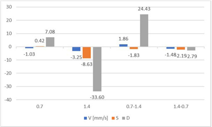
Figure 4 presents a comparison of the changes in the value of the average COP velocity and the both coefficients between the second and first half of the test for one selected participant. The values of the coefficient differences were obtained according to the scheme presented in Table 1, while the differences in the average COP velocities are the difference between the mean value of the average COP velocity obtained in the first and second half of the test.
Figure 4
Medians of the areas under the curve , lower and upper quartile and maximum and minimum values. Measurements with a frequency of scenery oscillations equal to: a) 0.7 Hz, b) 1.4 Hz, c) changing frequency from 0.7 Hz to 1.4 Hz, d) changing frequency from 1.4 Hz to 0.7 Hz. S – Sensitivity Coefficient, D – Balance Disturbances Coefficient
Discussion
Analysis of the results obtained for the whole group
When analyzing the medians of changes in mean COP velocity, one should first indicate higher values of this magnitude in the case of tests with moving scenery as compared to tests with eyes open and closed. A similar increase is noted in all such studies and was presented, among others, by teams led by Cunningham (Cunningham et al., 2006), Alahmari (Alahmari et al., 2014), Tossavainen (Tossavainen et al., 2003), or in previous studies conducted by the authors of this article (Jurkojć et al., 2017).
The division of the analysis of the results into the first and second half of the measurement allowed the determination of whether the measurement time has an effect on the change in the values of the recorded parameters (figure 2). The mean velocities of COP obtained for the constant oscillation frequency of the scenery indicate that the influence of the scenery is weaker in the second part of the measurement, suggesting that there is an effect caused by the participants getting used to the introduced disturbances. This is revealed by a statistically significant decrease in the medians of the mean values of COP velocity in the second half of the tests compared to the first half (from 12.4 mm/s to 9.3 mm/s at 0.7 Hz and from 9.8 mm/s to 9.2 mm/s at 1.4 Hz). Similar, statistically significant differences were not recorded in the case of tests performed with a changing frequency of scenery movement in the middle of the measurement. This may indicate that the change in the scenery movement parameters has reduced the effect of the subjects’ getting used to the introduced disturbances.
Figure 3 presents the medians of the areas under the courses of the determined coefficients – values determined using FFT and STFT, i.e. representing a signal in the frequency domain. First of all, it should be noted that body movement synchronized with the movement of the scenery was recorded for both frequencies of scenery movement – 0.7 Hz and 1.4 Hz; this is indicated by the non-zero values of the Sensitivity Coefficient. These results show that such movement also occurs at frequencies higher than those indicated by Cunningham and van Asten (van Asten et al., 1988; Cunningham et al., 2006), where the frequency of 0.5 Hz is described as the limit above which such a response of the examined subjects to the moving scenery disappears. The different results can be explained by the fact that the studies described in this paper were performed using an immersion system, in contrast to the quoted measurements which used the presentation of images on the screen.
By complementing the analysis in the time domain with values determined in the frequency domain, it can be seen that in the case of measurements carried out at a constant frequency, a decrease in the median value is observed in the second half of the measurement for both the Sensitivity Coefficient and Balance Disturbances Coefficient, while only changes in the Sensitivity Coefficient are statistically significant. This indicates that the habituation effect, suggested by the decrease in average COP velocity, is primarily due to a decrease in the movement of following the scenery, and to a lesser extent due to the subjects getting used to the moving scenery as a disturbing element of balance.
Particular attention should be paid to the results obtained during measurements with a changing frequency of the moving scenery. The analysis of the average COP velocity showed no statistically significant differences between the first and second half of the measurement. However, the analysis carried out in the frequency domain indicates that the change in the frequency of scenery movement affected the behavior of the subjects. In Figure 3c, it can be seen that the increase of oscillation frequency from 0.7 Hz to 1.4 Hz led to a decrease in the range of motion of the body synchronized with the movement of the scenery (reduction of the Sensitivity Coefficient). The opposite effect is visible when the oscillation frequency of the scenery is changed to a smaller one. Then, the Sensitivity Coefficient value increases, which means that the body movement component corresponding to moving with the frequency corresponding to the scenery movement also increased.
The above changes, when taking into account the lack of statistically significant differences in the average COP velocity, may indicate that there are changes in the amplitudes and/or frequencies of the cyclic components appearing by means of frequencies different than the scenery frequency, which should be checked by other mathematical tools not used in this research; the Balance Disturbances Coefficient was derived mainly to indicate to what extent the introduced disturbance has an influence on the ability to maintain one’s balance.
Case study – interpretation of the described coefficients
Frequency analyses can be used not only in scientific research on statistical studies for groups of people, but above all in everyday clinical practice when detecting and assessing possible imbalances in patients or trying to determine better training methods. In order to present the possibility of using such analyses in practice, the results of one of the subjects participating in the study were selected. For this subject, a combined analysis of the results determined in both the time and frequency domains was conducted (figure 4, tab. 2).
During the measurement performed at a constant frequency of 1.4 Hz, a decrease in the average COP velocity between the second and first half of the test was recorded. The simultaneous decrease in the value of both coefficients indicates that the lower velocity value results from both the smaller range of motion of the movement corresponding to following the scenery – a decrease in the Sensitivity Coefficient value – as well as from the better stabilization of the whole body that can be concluded from the lower Balance Disturbances Coefficient value. The overall result of this case of measurement can be interpreted as the subject getting used to the introduced disturbances. The difference in the Balance Disturbances Coefficient between the first and second half of the study also indicates the large destabilizing effect of the introduced disturbance at the beginning of the measurement, which was controlled to some extent during the measurement. It is worth noting here, however, that the obtained value of the Balance Disturbances Coefficient in the second half of the study is 30.98, which proves the persistent increased instability of the whole body.
Similar relationships as for the case involving a fixed frequency of scenery motion equal to 1.4 Hz can be observed when there is a change in the frequency of scenery motion from 1.4 Hz to 0.7 Hz. Here, too, there is a decrease in the value of the average COP velocity and both coefficients. The result obtained for this subject differs from the median results obtained for the whole group. This difference relates to the lower value of the Sensitivity Coefficient in the second half of the study in the analyzed subject, while for most subjects the value of this factor increases when the frequency changes to 0.7 Hz. In this case, the obtained result may suggest that the effect of getting used to the moving scenery was not disturbed by a lower frequency or that the frequency of 0.7 Hz affects the examined subject to a lesser extent.
In the test with frequency changing from 0.7 Hz to 1.4 Hz, an increase in average COP velocity is noticeable in the second half of the test. Changes in the values of both coefficients indicate that this increase in velocity is due to an increase in body instability (increase in the value of the Body Disturbances Coefficient), while the range of motion following the scenery decreased (decrease in the value of the Sensitivity Coefficient). This result, in combination with the values obtained during the measurement at a constant frequency of 1.4 Hz, shows that the frequency of 1.4 Hz has a larger destabilizing effect on the examined person. This is evidenced by the increase in the Balance Disturbances Coefficient in the second half of the measurement, when the 1.4 Hz frequency appeared.
The case of measurement at a constant frequency of 0.7 Hz seems to be the most difficult to interpret. There is a decrease in the average COP velocity with a simultaneous increase in the Balance Disturbances Coefficient and a nearly constant Sensitivity Coefficient. This discrepancy can be explained by the method of calculating the Balance Disturbances Coefficient, which is supposed to indicate how disturbed the stability of the examined subject is. A decrease in stability, as evidenced by an increase in the value of Balance Disturbances Coefficient, may occur with a simultaneous decrease in the value of average COP velocity. This may occur when the increase of the amplitude of cyclical components is observed with the simultaneous decrease of the frequency of these components. This phenomena cannot be observed only on the basis of time domain analysis.
Conclusions
Studies on the human body’s ability to maintain balance are very important both in sports training as well as diagnostic tests. These measurements are part of standard procedures in many centers and the method of testing them is still developing.
The use of moving scenery introduces a destabilizing element, which makes it possible to check not only the “static” condition – standing with eyes open and closed – but also the response to unbalancing factors. Such measurements are of great importance not only for people with balance problems, but also in sports training where trainers should very often be familiarized with player reactions to various stimuli.
The use of moving surroundings introduces an element that actively causes the destabilization of the tested subject, leading to additional movements of the whole body. These movements – natural in such conditions – makes the standard analyses based on the parameters determined in the time domain (such as the length of the COP path, average COP velocity or ellipse field) insufficient. This natural, additional movement increases the values of all these parameters both for healthy people and for people with problems with maintaining their balance. This fact impose the necessity of elaborating other methods of analyzing results, whereby one of them is analysis in the frequency domain – the method presented in this paper.
The use of calculations in the frequency domain enabled signal decomposition (decomposition of COP displacements) into cyclic components. The analysis of these components allows the authors to indicate the reasons for changes in the parameters determined in the time domain; the increase or decrease in the value of the time domain parameter can be explained and interpreted in terms of possible problems in maintaining one’s balance. The use of calculations in the frequency domain also made it possible to conduct an extended analysis of the impact of various parameters of the oscillating scenery on maintaining one’s balance. The gathered knowledge may be helpful in all kinds of sports where the ability to maintain one’s balance is crucial.
The presented methodology can be used in the development and verification of training methods as well as in the diagnosis of people with diseases impairing the ability to maintain their balance. Such analyses may indicate the existence or lack of a predisposition to practice a given sport discipline or indicate in which direction training should be conducted. In the case of medical applications, it seems advisable to carry out similar studies on groups of people with imbalances in order to determine whether there are certain elements characterizing given diseases.