Introduction
In recent years, determining the success criteria for soccer teams has been one of the prominent research topics in the scientific community (Bilek and Ulas, 2019; Kubayi and Toriola, 2020a; Young et al., 2019; Zhou et al., 2020). One of the main goals of sports science is to clarify the strategic performance objectives of teams and examine the indicators that improve their competitive outcomes (McGarry, 2009; Rizvandi et al., 2019). In this context, statistical analysis of team performance will provide soccer players and coaches with the opportunity to reevaluate their performance (Kubayi and Toriola, 2020a; Liebermann et al., 2002). Quantitative analysis of practice sessions can play an important role in detecting priority areas in training of the team, and is a crucial step in observing the opponents’ general characteristics, especially their strengths and weaknesses. Soccer is a large and comprehensive industry and, in recent years, has been the subject of numerous statistical estimation studies. Previous studies on soccer match prediction focused on key attributes of the games such as taking possession of the ball (Aquino et al., 2019; Kubayi and Toriola, 2019; Lago-Peñas and Lago-Ballesteros, 2011), accurate passes (Kubayi and Toriola, 2020b; Lago-Ballesteros et al., 2012), game interruptions (corners, touches, etc.) (Bilek and Ulas, 2019; Siegle and Lames, 2012), and to a more limited extent, defensive and offensive performance variables (Almeida et al., 2014; Ismail and Nunome, 2020). Also, since soccer is a low-scoring sport, there were many studies showing that scoring the first goal affects the match outcome (Armatas et al., 2009; Bilek and Ulas, 2019; García-Rubio et al., 2015). There are many variables which determine the success criteria of soccer teams. It has become inevitable to use statistical techniques that allow visualization of these variables to evaluate them together. However, there is a gap in this area in the literature.
Variables discussed in the literature are generally divided into two classes: notational (aerial challenges, dribbles, losses of control, passes, tackles, and times tackled, etc.), and situational (quality of opposition, game location, match status). In previous studies, various practical applications have been established from the examination of the in-game variables (notational) of the winning, losing or drawing teams. While Tenga et al. (2010a, 2010b) indicated that counterattacks were effective against weak defences compared to normal attacks, Lago-Peñas et al. (2010) and García-Rubio et al. (2015) showed that winning teams attempted more shots at the goal. Additionally, possession of the ball was a decisive variable among the teams that won, lost, or drew.
Various performance studies have investigated the quality of opposition (stronger, weaker or balanced), as among the most important elements of situational variables (Bilek and Ulas, 2019; Lago, 2009; Liu et al., 2016a; O’Donoghue, 2009; Taylor et al., 2008). Taylor et al. (2008) classified the opposition teams as stronger or weaker using clustering analysis. Bilek and Ulas (2019) predicted match outcomes for the premier league by correlating these with the relative quality of the opposing teams. The complex and dynamic environment of soccer poses several difficulties in measuring performance of the team (Vilar et al., 2012). Therefore, visualizing these performance indicators together will reduce this complexity. In addition to interpreting performance indicators separately, the present study aimed to visualize how variables behave together with the help of multidimensional scaling (MDS) analysis, depending on the quality of the opposition. This analysis will help the audience understand the complex structure created by many variables and contribute to the literature.
Previous studies revealed the importance of modelling in improving the estimation of team performance and achievement. In forecasting studies, an important consideration is the identification of variables that affect emerging models. In such an evaluation, using decision trees with multivariate statistical methods, such as MDS and clustering analysis, constitutes important tools in understanding the structural issues (Moura et al., 2014). Multivariate statistical methods encompass matrix algebra, statistics, and geometry. These methods are useful to analyse multivariate differences between groups, by revealing the behaviour of multiple variables, and detecting similar or dissimilar patterns among structures (Green, 2014). In addition, decision trees, MDS, k-means, and one-way ANOVA are used to analyse the variables that impact match results.
The main purpose of this study was to predict the win, loss, and draw positions of the teams using twenty in-game variables (accurate passes, aerials won, clearances, corners, defensive aerials, lost balls, dribbles attempted, dribbles past, dribbles won, fouls, interceptions, key passes, offensive aerials, offside, shots on target, successful tackles, tackles attempted, total passes, total shots, touches), together with the quality of the opposition (stronger, balanced and weaker) as a situational variable and the scoring first variable (categorical). The structural components of teams, which constituted stronger, weaker, and balanced opponents, were modelled using various graphical methods.
Despite similar studies on this subject in the literature, using MDS analysis to determine and visualize the relationship between the performance indicators that affect the match outcome was the novel part of the study.
Methods
Sample and Variables
Match performance data consisted of all Champions League matches between the 2010/2011 and 2019/2020 seasons (10 years), and the data used in the study were taken from whoscored (“WhoScored.com,” 2020), which is the public accessed website of OPTA Sportsdata company (Lorenzo-Martínez et al., 2020). Liu and colleagues (2013) found that the inter-operator reliability of the tracking system used by this company was acceptable, and the intra-class correlation coefficient was strongly significant (ranged from 0.88 to 1.00). There were a total of thirty-two teams in the Champions League each season and each team played six matches in the group stage, thus 192 (32×6) observations per season, and the total number of results in the ten years was 1920 (192×10). The match result, which was our dependent variable, was divided into three groups as ‘win’, ‘draw’ and ‘loss’ in the dataset. In the study, we used a total of twenty variables, including three situational variables (match outcome, quality of the opposition, and match location), and the seventeen statistically significant performance indicators identified by one-way ANOVA. The variables used in the study are given in Table 1.
Table 1
Variables in the study and their description
One-way ANOVA, using all matches in the group stage for the Champions League between 2010-2011 and 2019-2020 (a 10-year period), was applied to the twenty performance indicators. The k-means clustering analysis was conducted using variables (seventeen performance indicators) that were statistically significant from the one-way ANOVA results, which classified Champions League teams as either strong, weak, or balanced. Variables that impacted these classes were analysed using two-dimensional MDS maps, which indicated that teams playing against stronger, weaker and balanced opponents had different structures in terms of performance indicators. Finally, the probability of teams wining, losing, or drawing, according to their classification, was estimated on seventeen in-game variables (notational) using decision tree analysis.
Performance indicators in this study included variables related to the match outcome given in Table 1, and the operational definitions of these variables have been provided in previous studies (Liu et al., 2015a, 2016a). Since the reliability of these variables has been proven in previous studies (Castellano et al., 2012; Kubayi and Toriola, 2020a; Lago-Peñas et al., 2010, 2011; Liu et al., 2013, 2015a), the reliability test was not applied again in our study.
In this study, due to the different structure of other rounds, we only used data from the group stage. Qualifying and final rounds can also be analysed, but we thought that 2-legged matches should be evaluated differently to matches in the group stage. Similarly, García-Rubio et al. (2015) analysed the group stage and the knockout phase differently. Additionally, the goals for and against were not used in the analysis as they directly affected winning the match and would result in the dominance of other situational variables and performance indicators in the decision tree analysis.
Statistical Analyses
First, the mean and standard deviation values, which were the main statistical performance indicators, were calculated, taking into account the variability of match results (win, draw, and loss) being the dependent variable. One-way ANOVA determined which performance indicators were significant, together with the significant F values, pairwise comparison, and a Tukey HSD test to reveal differences between groups (Salkind, 2010). Results of one-way ANOVA and Tukey HSD multiple comparisons are summarized in Table 2. Additionally, the effect size value, being the magnitude of the difference between the null hypothesis and the alternative hypothesis, was calculated. Eta squared (an effect size measure used to represent the standardized difference between two means) has the same effect size classes as Cohen's d when there are more than two groups. However, the range values of the classes are different than Cohen's d. Eta squared takes a value between [0, 1], with the effect size being interpreted as: non-significant (≤0.009), small (>0.01, <0.0588), moderate (≥ 0.0589, <0.1379, and large (≥ 0.138) (Tomczak and Tomczak, 2014). A small effect size would require large sample sizes. Huge sample sizes can detect differences that are quite small and probably trivial (Sullivan and Feinn, 2012). In this study, small effect sizes were acceptable because the sample size was large.
Table 2
One-way ANOVA and Tukey HSD tests results by the match outcome
[i] * symbol indicates a statistically significant difference at the 95% confidence level ‡,†,● symbols show the Tukey HSD test results. The same sign in both groups in a row indicates that the two groups are different from each other. Two different symbols in one group mean that this group is different from the other groups. If groups are different from each other, the group with the higher average is superior.
The data set was divided into three main parts in order to compare the overall performance of the teams in more detail, observe the elements comprising the main structure of the opposing team, and examine the effects of the decision-making system. The data were partitioned into three categories, ‘playing versus a stronger opponent’, ‘playing versus a weaker opponent’ and ‘playing versus a balanced opponent’, using the k-means clustering method (k = 3). The first group whose distance to the cluster centers was less than 0.179, was classified as “weaker” (n = 795). The second one contained the group whose distance to the cluster centers was between 1.8 and 1.223, and this group was called “balanced” (n = 787). The third group consisted of “stronger” in which the distance from cluster centers differences was higher than 1.224 points (n = 338). The main purpose of the cluster analysis was to reveal similarities and dissimilarities between clusters (groups) (Everitt et al., 2011). With the clustering analysis, the structure variables that changed the performance of the teams were seen more clearly.
As part of multivariate statistical analysis, MDS, utilized in the literature to support clustering analysis results (Kruskal, 1977; Lawless, 1989), maps the variables on a two-dimensional coordinate system according to their similarity and dissimilarity (Kruskal, 1964). In this study, different MDS maps were performed for teams according to the quality of the opposition. Our purpose in these maps was to identify which variables had similar characteristics for teams playing against ‘stronger’, ‘weaker’ and ‘balanced’ opponents. To make the findings on the map easier and more coherent, k-means clustering analysis (k = 3) was applied on MDS maps, demonstrating how the performance indicators affected the team. Using MDS and k-means clustering analysis together clarified the purpose of the study in using the decision tree method.
The decision tree algorithm was applied to each set of match results (according to the quality of the opposition). This graphical decision-making method consists of branches and nodes, divided into subcategories with different effects, to establish classification accuracy. Variables that have the most effect on the match results are seen with the decision tree. All analysis was controlled at the 95% significance level.
All statistical analyses were performed using R statistical software. ‘Stats’ and ‘MASS’ libraries in R software were used for MDS and k-means clustering analysis (Team, 2017). The radar chart was applied in the R program with the ‘ggradar’ library. ‘Rpart’ and ‘rpart.plot’ functions were used for the decision tree (Milborrow, 2017; Therneau et al., 2010).
Results
The results of one-way ANOVA and Tukey HSD tests to determine the performance indicators affecting the outcomes of matches are provided in Table 2, together with the effect size values. Lost balls, interceptions, and successful tackles variables were the only ones which did not present a significant difference according to the match outcome. As an example, accurate passes differed significantly as means compared to the match outcome (p = 0.000*). All groups had two symbols, thus were statistically different from each other. The winning teams were characterized by more accurate passes than the drawing and losing teams. Similarly, drawing teams had more accurate passes than losing teams. As a result of one-way ANOVA for this variable, the effect size value was estimated as moderate.
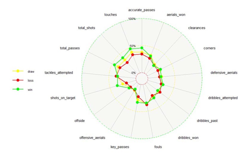
One-way ANOVA was performed to determine the variables that affected the outcome of the match. A radar chart was used to better understand these variables and visually identify superior groups for each performance indicator (Figure 1). The winning teams were superior to the drawing and losing teams in many performance indicators, however, losing teams were superior in dribbles past, fouls, and tackles attempted.
Match performances of the teams may differ according to the quality of the opposition. Thus, one-way ANOVA and k means clustering analyses (k = 3) were applied, using statistically significant variables to determine three clusters. The resulting clusters were described as those who played against weaker opponents (n = 338), those who played against balanced opponents (n = 787), and those who played against stronger opponents (n = 795). MDS analysis was performed for each type of the opponent to examine how the performance indicators of the three clusters differed. Figure 2 shows the graph of MDS analysis applied for teams playing against weaker opponents. Teams that played against weak opponents had very similar performance indicators highlighting ball possession, such as accurate passes, total passes, and touches. Similarly, teams playing against weaker opponents were similar to each other considering attacking features, such as corners, key passes, shots on target, and total shots.
Figure 2
MDS analysis result graph for teams playing against weaker, stronger, and balanced opponents
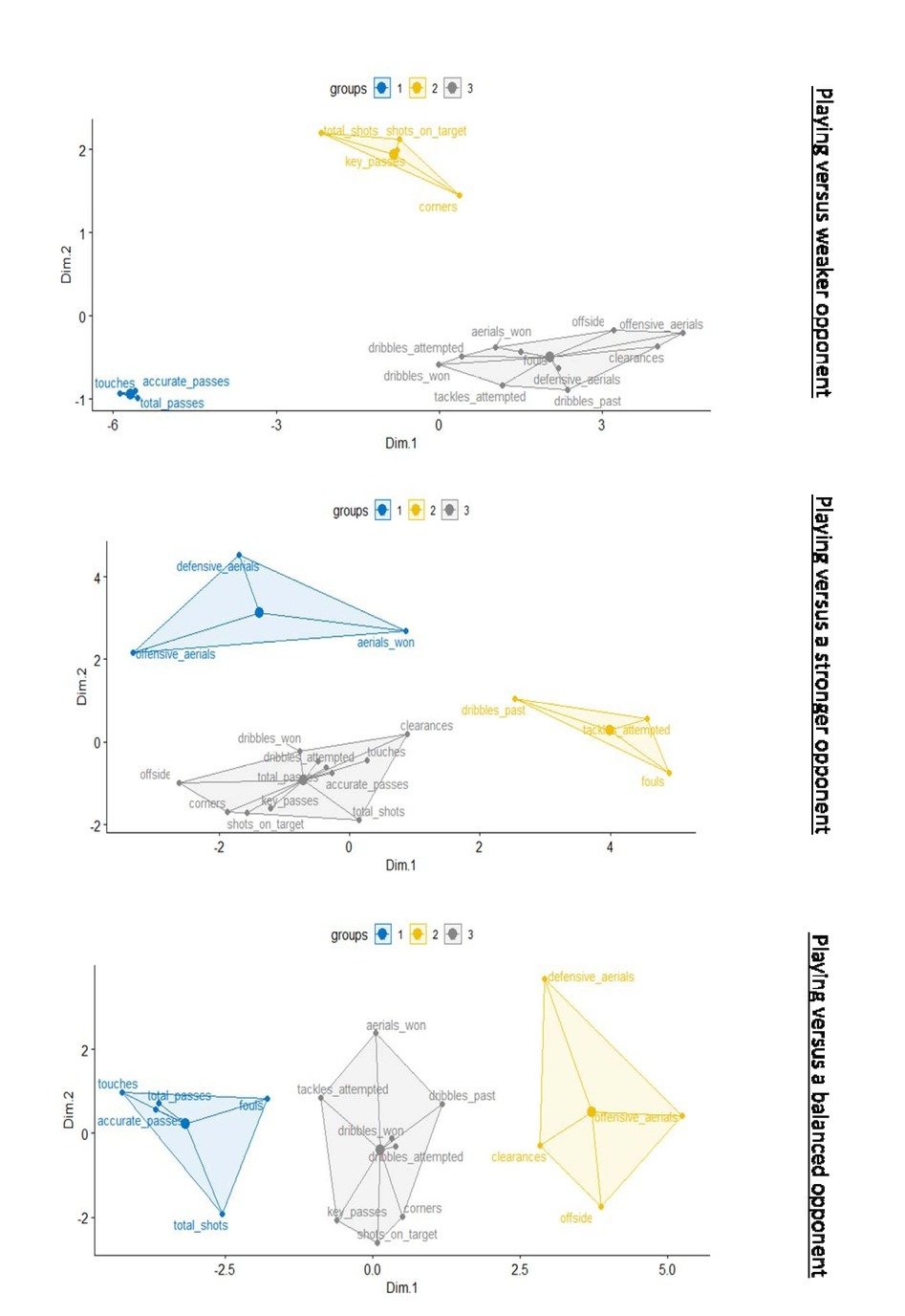
The MDS analysis for teams playing against stronger opponents is given in Figure 2. The defensive aerials, offensive aerials, and aerials won indicators resemble those of teams playing against stronger opponents. In addition, teams that played against strong opponents, in terms of dribbles past, fouls, and tackles attempted, had similar characteristics to each other. While reviewing the one-way ANOVA results and the radar chart (Figure 1), we stated that losing teams had higher values than winning and drawing teams in terms of these three performance indicators (dribbles past, fouls, and tackles attempted). This is a proof that the analysis provided consistent results.
Mapping performance indicators for teams playing against balanced opponents (Figure 2) indicated a more balanced structure compared to strong and weak opponents. These indicators (accurate passes, total passes and touches, the total shots and fouls) for teams that played against weak opponents were similarly grouped to those of balanced teams.
The three MDS maps of stronger, balanced, and weaker competitors highlight different structures of performance indicators. For teams that played against weak opponents, performance indicators such as accurate passes, touches, and total passes, had a very similar structure. In addition, for teams playing against strong opponents, performance indicators, such as dribbles past, fouls, and tackles attempted, had similar features to each other. The radar chart in Figure 1 indicates these variables had higher values in losing teams. Therefore, it was clear that teams playing against strong opponents had common features with losing teams.
Decision tree analysis was applied separately to each cluster (weaker, stronger, and balanced opponent), identified by k-means clustering analysis using statistically significant performance indicators (from one-way ANOVA), match location, and situational variables.
In the decision tree analysis, each node has three proportions representing draw (yellow), loss (red), and win (green), respectively, and is coded according to relative size. The percentage of each node is given below these rates. The left decision is yes, and the right is no; that is, if the condition under the node is met, it must be continued on the left side, or conversely on the right side.
The decision tree for teams that played against stronger opponents (Figure 3) indicates that chances of winning and losing were 0.27 and 0.50, respectively. If teams playing with stronger opponents scored the first goal, they had a 0.59 chance of winning the match, indicating that teams playing with stronger opponents could double the probability of winning by scoring the first goal. The chances of losing when they failed to score the first goal increased to 73%. The probability of winning was only 6%. In addition, when the shots on target were less than 6, the probability of losing increased to 0.78.
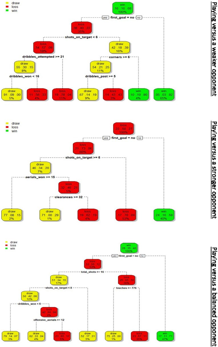
Figure 3 shows the decision tree performed for teams playing against weaker opponents. Those teams had a 68% chance of winning the match. This increases to 92% if they scored the first goal. Thus, the probability of losing the match was only 0.03 when a team playing against a weaker opponent scored the first goal. If they failed to score the first goal, the odds of winning were 0.22. However, if shots on target were more than 6, and corners were 6 or less, the chances of winning rose to 80%. If the team who played against a weaker opponent, failed to score first, the shots on target were less than 6, and the dribbles attempted were less than 21, the probability of losing the match increased to 78%. Furthermore, if the conditions in the top nodes were met, the probability of a draw was 91% if the dribbles won were less than 16, and the probability of a draw was 11% when there were more than 16 dribbles won. Similarly, when the dribbles past were more than 5, the team was more likely to draw (0.67), and when they were less than 5, it was more likely to lose (0.43).
Figure 3 shows a decision tree for teams playing against a balanced opponent, who had a 0.40 probability of winning a match. When they scored the first goal, the probability of winning was 0.71, while failing to score the first goal reduced their chances of winning to 0.12. If they failed to score the first goal and the total shots were less than 16, the probability of losing increased from 0.35 to 0.65. Additionally, if touches were less than 776, the probability of losing increased to 67%. If the conditions in the top nodes were met, the probability of losing the match was 0.33 if the offensive aerials were more than 12, but decreased to 0.65 when they were less than 12.
Discussion
The aim of the study was to statistically analyse performance indicators and situational variables using MDS as a novel visualization approach, based on the quality of the opposition, that significantly affected the outcome of the match in the Champions League group stage. The present study analysed teams' performance and situational variables based on a large sample (1920 matches from the UEFA Champions League) and hence in a more detailed way than previous research (Bush et al., 2015; Liu et al., 2016b; Yi et al., 2020).
Firstly, one-way ANOVA, Tukey HSD, k-means clustering, and decision tree analyses were applied, with radar graphs for data visualization. In addition to these methods, the investigation of used variables considering performance of teams’ variation may contribute to better interpretation and understanding with the help of MDS.
The influence of scoring the first goal, which is one of the most important findings of our study, has been highlighted in several investigations. Scoring the first goal has been mostly analysed from the perspective of its effect on the match outcome (Armatas et al., 2009; Michailidis et al., 2013; Molinuevo and Bermejo, 2012). Soccer is a low-scoring team sport, and the number of goals scored per match in the top four leagues in Europe (Premier League, Bundesliga, Calcio, and La Liga) was 2.66 (Anderson and Sally, 2013). Sports where the final score is low, such as soccer or ice hockey, show the importance of scoring the first goal (García-Rubio et al., 2015; Jones, 2009). Armatas et al. (2009) and Molinuevo and Barmejo (2012) also concluded that teams who scored first presented a higher probability of winning a match. Conclusions of this study established the importance of scoring the first goal for teams for the UEFA Champions League. Teams playing against stronger, balanced, and weaker opponents had a 0.59, 0.71, and 0.92 chance, respectively, of winning the match if they scored the first goal. Other studies which focused on the UEFA Champions League (García-Rubio et al., 2015), five major European leagues (Lago-Peñas et al., 2016) and the England Premier League (Bilek and Ulas, 2019) support our findings.
Another important performance indicator affecting the match outcome was shots on target, located in the decision tree of the three types based on the quality of opponents. For teams competing against weaker, balanced and stronger opponents, shots on target increased chances of winning by 0.14, 0.16, and 0.17, in the ranges ≥ 6, > 8, and > 6, respectively. Our findings are in line with studies which revealed that shots on target might have essentially positive impact on the chance of winning (Liu et al., 2015b, 2016a; Mao et al., 2016; Moura et al., 2014; Zhou et al., 2018). A previous study indicated the usefulness of this explanation in the match situation of low-level teams when playing against similar opposition levels (Liu et al., 2016a). In addition to this study, we found that whatever the quality of the opposition, shots on target increased the probability of winning. Considering the huge influence of shots on target, coaches should design practice sessions where the attention is paid to shooting accuracy (Zhou et al., 2018).
Other important variables apart from scoring first and shots on target which affected the match outcome were as follows. For teams playing against strong opponents, an increase in performance indicators, aerials won and clearances, increased their probability of winning, whereas, for teams playing against weak opponents, dribbles attempted increased the chance of winning. Conversely, corners, dribbles won, and dribbles past had a negative effect on the chances of winning. Previous studies support our findings because these performance indicators were adequate to predicted match outcomes by the level of the opposition (Lago, 2009; Liu et al., 2015a; Taylor et al., 2008).
On the other hand, the match location was shown as one of most important variables which affected winning in many studies in the literature (Lago-Peñas et al., 2016; Taylor et al., 2008). In contrast to these studies, the match location was included in the decision tree analysis for teams that played against strong, weak, and balanced teams, however, no effect was observed. This divergence may be due to the stronger competitiveness of the UEFA Champions League compared to the domestic leagues as teams seek to perform at the highest level possible in this tournament (Yi et al., 2020).
The results of this paper should be assessed in the light of a number of implications and limitations. The detailed assessment and comparison of the impact of the quality of the opposition, performance indicators, and the match outcome on UEFA Champions League performance using multivariate statistical approaches within this paper suggests several implications for coaches. By forming visual analyses of teams with performance-related indicators, the opposition can be studied, and results may help develop different tactics and choose the player before the match according to the quality of the opponent. The collective structure of all performance indicators was visualized by MDS analysis according to the quality of the opposition. We believe this situation will be important for coaches to develop different tactics and choose best players before the match according to the quality of the opponent.
The current study has some limitations that should be reviewed to develop the practicality of its results and need to be considered in forthcoming applications. Firstly, for a more improved and comprehensive review of the output, the cards in the match (yellow and red), the individual player performances and positions can be added to the study. Secondly, the knockout stage of the championship may change the match outcome and performances which was not included in this stage. Also, these visual methods along with other statistical methods can be applied to match periods (such as the first and the second half, 0-15 min, 16-30 min, 31-45 min, etc.). This study methodology should be supported and verified in different leagues and tournaments (UEFA Europa League, Premier League, La Liga, Bundesliga, knockout stages, etc.) in future works.
Conclusions
In conclusion, this study shows that performance indicators and situational variables differ for winning, drawing, and losing teams in the UEFA Champions League group stage. It highlights the match outcome evaluated according to the quality of the opponent. In addition, it proves that performance indicators in a match have different structures according to the quality of the opposition. Performance indicators which indicate air dominance (such as defensive aerials, offensive aerials, and aerials won) in teams playing against stronger opponents, differ from the other groups. Similarly, it was determined that performance indicators involving possession of the ball such as accurate passes, total passes, and touches, in teams playing against weaker opponents differ from the others. In teams playing against balanced opponents, performance indicators are most balanced. Regardless of the quality of the opposition, however, performance indicators of scoring first and shots on target, increase chances of winning for all groups. These findings can help coaches develop different strategies based on the opponent's quality, situational variables, and performance indicators before or during a match.