Introduction
Team sports are social systems (Araújo and Davids, 2016; Parlebas, 2002) in which teammates collaborate (i.e., positive interaction) to overcome the opposing team (i.e., negative interaction). Thus, team sports are complex systems in which players should respond to the uncertainty due to social interaction, and, in some sports, to the interaction with the environment (Araújo and Davids, 2016; Newell, 1986; Parlebas, 2002). The interaction between players is determined by the social structure (e.g. number of players per team), configuration of the space (e.g., the relative pitch area per player), traits of time (e.g., duration), and use of the mobile object (e.g., type of the ball used) of each team sport. The structural traits (Newell, 1986; Parlebas, 2002), characteristics of players, situational variables and strategic decisions of coaches determine the collective tactical behaviour of teams (Castellano et al., 2016; Silva et al., 2014).
Players´ collective tactical behaviours have been analysed by positional data for more than 15 years in team sports (Low et al., 2020; Rico-González et al., 2020). With this aim, collective tactical variables have been classified into three principal groups (Rico-González et al., 2019): a) the central position of several players (i.e., geometrical centre [GC]), b) the distance between players or between players and reference points (i.e., dyads), and c) the use of space (Low et al., 2019; Rico-González et al., 2019). The GC represents relative positioning of each team in forward-backward and side-to-side movements using a single point only (i.e. x and y coordinates) (Araújo and Davids, 2016) and it was suggested for assessing the coordination among the whole team and between two teams’ movements (Frencken et al., 2011). The distance variables represent the distance between two points inside the playing area (i.e. player-player; player-goal, player-space, player-ball) and have been used to assess the relationship between players or groups of players and the distance of the players to specific zones within the playing space (Rico-González et al., 2020). The area variables assess the management of the space by a player or several players at each point in time or take into account the entire training task or match (Bueno et al., 2018; Frencken et al., 2011; Moura et al., 2016; Olthof et al., 2018). In addition, these tactical variables can be assessed according to the numerical relation of players (Low et al., 2019). As with the other tactical variables, the measurement of the use of space can be interesting in both training and competition. Team sports coaches can analyse the influence of the manipulation of the structural traits on tactical behaviour (Coutinho et al., 2018; Gonçalves et al., 2017; Olthof et al., 2018; Timmerman et al., 2017; Travassos et al., 2018) to design and select training tasks that force players to use the playing space similarly as in the match situation. In addition, the measurement of the use of space allows for assessment of the effects of training interventions at the tactical level (Coutinho et al., 2018). Also, it makes possible the examination of the use of space during competition and the comparison to the formation used by the team during the match (Memmert et al., 2019).
Gréhaigne (1992) proposed the assessment of the use of space in team sports more than 25 years ago. Specifically, the author suggested measurement of the effective play-space in soccer (Gréhaigne, 1992). Later, several authors proposed and measured different variables to assess the use of space in team sports (Low et al., 2019; Rico-González et al., 2019). In addition to tactical position and distance variables, a recent systematic review provided a comprehensive summary of tactical variables used to analyse the use of space in soccer, with a particular focus on organising the methods (Low et al., 2019). However, to our knowledge, no study has identified the original spatial tactical variables nor has assessed their conceptual and computational modifications in team sports. This type of study would allow assessment and understanding of the proposal of new tactical variables and their conceptual and computational modifications at a practical level to analyse the use of space in team sports. Since team sports are complex systems, in addition to traditional methods of linear analysis (Low et al., 2019), it would be interesting to identify the nonlinear tools used to analyse the predictability of the use of space in team sports. Therefore, the aim of the review was to identify spatial tactical variables employed to assess the use of space in team sports by analysing positional data. In addition, the computational methods were examined, a critical assessment was carried out and future considerations were suggested.
Methods
Search Strategy
The systematic review was prepared in accordance with the Preferred Reporting Items for Systematic Reviews and Meta Analyses (PRISMA) guidelines (Moher et al., 2009). The protocol was not registered prior to initiation of the project and did not require Institutional Review Board approval. A systematic search of four databases (i.e. SPORTDiscus, PubMed, ProQuest and Web of Science) was performed by three authors (MRG, ALA, JPO) to identify articles published before the 13th of November, 2018. The authors were not blinded to journal names or manuscript authors. To provide an explicit statement of question, the PICO (Moher et al., 2009) design was used. The search was carried out using two filters when the database allowed it: journal article; and title (TI)/abstract. This was possible in all databases except for Web of Science, which was searched through the text. In addition, in the final database, the sports sciences branch was selected. Database search strategy considered three main groups: 1) population, team sports (at least two players per team and, in which the use of the mobile object was simultaneous), 2) intervention, the assessment tools were included, and 3) outcomes, the results that the authors hoped to find. The keywords were connected with “AND” to combine the three groups and using “OR” to link the words of each group (Table 1).Screening Strategy and Study Selection
Table 1
Database search strategy
When the authors had completed the search, they compared their results to ensure that the same number of articles were found. Then, one of the authors (MR) downloaded the main data from the articles (title, authors, date, and database) to an Excel spreadsheet (Microsoft Excel, Microsoft, Redmond, USA) and removed the duplicate records. Subsequently, the same authors screened the remaining records to verify the inclusion-exclusion criteria using a hierarchical approach (Table 2) in two phases: 1) Phase 1, where possible, titles and abstracts were screened and excluded by two authors (MR, ALA) and 2) Phase 2, full texts of the remaining papers were then accessed and screened by the same two authors (MR, ALA).
Table 2
Inclusion/exclusion criteria
Table 3
Collective area variables in team sports
| Study | Variable / Computation | Sport | Competition Level | Task | Main results |
|---|---|---|---|---|---|
| Collective occupied space variables | |||||
| Okihara et al. (2004) | Team area*^ The quadrilateral formed by the four outfielders | Futsal | Professional | Match | The transition between offense and defence may be explained from the fact that offence is done in a small |
| Team area^ The dimension of a square = length (between the front and the tale)* width (between the left-edge player and the right- edge player) | Soccer | Professional | Match | area and that opponent defence is done in a large area in this situation. As a result, the ball is taken from each other easily, which leads to the frequent change in offence and defence. | |
| Frencken and Lemmink (2009) | Surface area is the total field coverage of one team Area (m2) *^ | Soccer | Young | 4+GK vs. 4+GK | In five out of nine goal-scoring opportunities, a sudden increase in the surface area for the attacking team or a decrease in the surface area of the defensive team was found. |
| Frencken and Lemmick (2011) | Surface area^: the area within the convex hull. CH: modified Graham algorithm (Graham, 1972). [CA(t)]: the area was calculated by adding the triangles of consecutive points of the CH and the centroid | Soccer | Young | 4+GK vs. 4+GK | The aim was to establish an overall linear association per game for surface areas of two teams. The results were near zero for three games (0.03, 0.07 and 0.01). This implied no linear association for the surface areas of the teams. |
| Duarte et al. (2012) | Surface area^: the area of a triangle Area: Area (A, B, C): abs((xB*yA-xA*yB) + (xC*yB-xB*yC) + xA*yC-xC*yA))/2 | Soccer | Young | 3+GK vs. 3+GK | Analysis of the surface area of each team did not reveal a clear coordination pattern between subgroups. But the difference in the occupied area between the attacking and defending subgroups significantly increased over time. Findings emphasized that major changes in sub-group behaviors occurred just before an assisted pass was made (i.e., leading to a loss of stability in the 3 vs. 3 sub-phases). |
| Moura et al. (2012) | Coverage area^: the area that a team covers CH: Quickhull technique (Barber et al., 1996) [CA(t)]: they divided the team convex hull into triangles. Then, they summed the areas of all triangle within the convex hull | Soccer | Professional | Match | While the players attacked, the area ranged from 905 ± 4 to 1,407 ± 6 m2, respectively. On defence, the values were smaller (p. 0.05) and ranged from 774 ± 5 to 1,158 ± 6 m2 for the area. In defending circumstances, the teams presented a greater area when they suffered shots on the goal than when the teams performed tackles. In attacking situations, the teams presented a greater area when they suffered tackles than when they performed shots on the goal. |
| Clemente et al. (2013) | Effective free-space: the real area that a team covers without intercepting the effective area of the opposing team. The GK was considered. Triangles as the combinations of the total number of players within a team | Soccer | Young | 7+GK vs. 7+GK | Without the ball possession, the team was able to generate seven effective triangles. This effective triangulation was based on the inter-player distances. This kind of defence was difficult for the opposing team to overcome since it does not leave much free space to play. |
| Bueno et al. (2018) | Surface area^ normalized by the maximum possible value that a team can present on the court The surface area was represented by the CA(t), calculated from the position of the players of the same team. CH: their vertices were calculated using quickhull technique (Barber et al., 1996) [CA(t)]: their vertices were calculated using quickhull technique (Barber et al., 1996) | Futsal | Young and professional | Match | While the players were attacking, all categories presented a greater surface area, compared to values when players were defending. Among the categories, the results showed lower area values for the younger players. The surface area results showed different forms of organization for each of the categories in specific situations of shots on goal and interceptions. |
| Collective influence space variables | |||||
| Yue et al. (2008) | Major range of GC | Soccer | Professional | Match | The authors reported the concept and represented it graphically. |
| Collective dominant space variables | |||||
| Taki and Hasegawa (2000) | Dominant region: the region where the individual can arrive earlier than any other individual when starting at t. | Soccer | Professional | Match | The study reported the concept and this has been applied to team sports. |
| Fujimura and Sugihara (2005) | Weighted dominant region area○: player’s weighted dominant area was obtained by summing the weighted pixel values in his dominant region Dominant area weighted by the goal: higher scores are given to points nearer to the goal Dominant area weighted by the ball: higher scores are given to points nearer the ball. | Field Hockey | - | Match | The nearer the position to the goal or to the ball, the higher the weighted area, but by using only these indices we cannot evaluate the contribution of players whose position is far from the goal and the ball. |
| Fonseca et al. (2012) | Voronoi cells: division of the plane by means of the assignment of the points of the field to each player which are closer to that player than any other. | Futsal | Senior | 5-v-4+Gk | Compared to defenders, larger dominant regions were associated with attackers. Furthermore, these regions were more variable in size among players from the same team but, at the player level, the attackers’ dominant regions were more regular than those associated with each of the defenders. |
| Fonseca et al. (2013) | Superimposed Voronoi Diagram (SVD): Superimposition of the Voronoi diagrams of the two teams. Maximum percentage of overlapped area (Max%OA): maximum percentage of that player’s Voronoi region covered by the Voronoi region of an opponent; and Percentage of free area (%FA): the remaining space | Futsal | Senior | 5-v-4+Gk | The observed patterns of behavior, assessed by means of the % of free area, lean more towards low levels of exclusive dyadic interaction (% of free area values inside the interval (0.22, 0.50) %), which was expected as defense players were playing in a zone defense fashion due to their numerical disadvantage. |
[i] GK: Goalkeeper; ○: As Taki and Hasegawa (2000) they also considered the time instead of the distance. However, they did not assume that each player’s acceleration was constant and considered a resistive force that decreased the velocity.
*: The mathematical method to determine the metric was not provided; ^: excluding goalkeeper; [CA(t)] Convex hull area at each instant of time t.; GC: geometrical centre
GK: Goalkeeper; ○: As Taki and Hasegawa (2000) they also considered the time instead of the distance. However, they did not assume that each player’s acceleration was constant and considered a resistive force that decreased the velocity.
*: The mathematical method to determine the metric was not provided; ^: excluding goalkeeper; [CA(t)] Convex hull area at each instant of time t.; GC: geometrical centre
In comparison to Low et al. (2019), we did not include several tactical variables as the stretch index (Yue et al., 2008) and the team spread (Yue et al., 2008). As those authors themselves pointed out, these variables may not be computations of the area per se (Low et al., 2019). In the same way, we did not consider tactical variables that assessed the numerical relations of players within pre-established sub-areas (Clemente et al., 2015; Low et al., 2019; Vilar et al., 2013) because this space was not calculated through the data position of players. Moreover, we did not consider variables that analysed the use of space for players in isolation (e.g., players´ mayor range, spatial index exploration [SEI]) because these variables were not “collective” tactical behaviours (Table 2, 5th inclusion/exclusion criteria).
Any disagreements on the final inclusion-exclusion status were resolved through discussion in both the screening and excluding phases. Moreover, relevant articles not previously identified were also screened in an identical manner and the studies that complied with the inclusion-exclusion criteria were included and labelled as ‘not identified from search strategy’.
Results
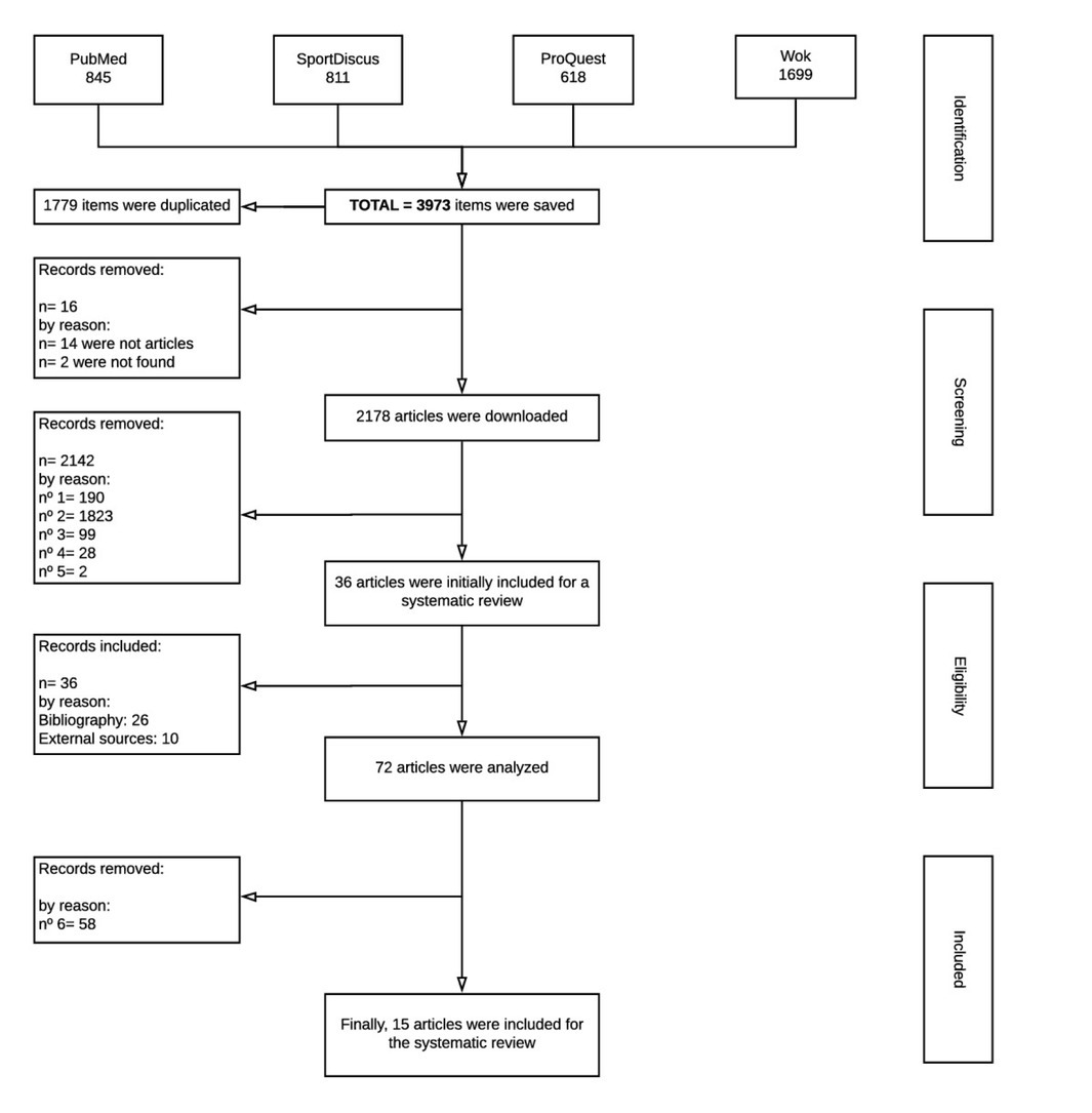
A total of 3973 documents were initially retrieved from the aforementioned databases, of which 1779 were duplicates. Thus, a total of 2194 original articles were screened. Next, the titles and abstracts were verified against criteria 1-6 and studies were excluded where possible: criterion 1 = 190 studies; criterion 2 = 1823 studies; criterion 3 = 99 studies; criterion 4 = 28 studies; criterion 5 = 2 studies. The full texts and abstracts of the remaining articles were screened to apply the inclusion/exclusion criteria, leading to exclusion of 2142 articles. A further 14 records were removed as they were not articles and another 2 were not found. Therefore, 36 articles were initially included in this review. In addition, while reviewing references of the included articles, the authors found and added 36 articles that met 1-6 inclusion criteria. In most of these studies, the search tool (group 2) was not detailed in the title or the abstract. Therefore, 72 articles were analysed and 58 of them did not fulfil inclusion criterion 6. Finally, 15 articles were included in this systematic review (Figure 1).
Discussion
The aim of the review was to identify spatial tactical variables employed to assess the use of space in team sports utilizing positional data. In addition, computational methods were examined, a critical assessment was carried out and future considerations were suggested. The main findings were that: a) spatial team sports tactical variables could be classified into 3 principal types: occupied space, exploration space and dominant/influence space; b) most of the occupied space tactical variables did not consider GKs and the rest playing space to assess the occupied space, but several studies have proposed new variables that considered the total playing space (i.e. effective free-space, normalized surface area); c) only a collective exploration space variable has been suggested: the major range of the GC; d) the dominant/influence space has been based on the Voronoi region while several studies based their computation on the distance d and others suggested the use of the time (t); e) four different techniques (i.e. SampEn, cross-SampEn, ApEn, ApEnRatioRandom) have been used to assess the predictability of the use of space; and f) the lack of consensus on computation methods and techniques to assess the use of space and its predictability made it difficult to compare studies.
Occupied space
Gréhaigne (1992) suggested the effective playing-area (EPS), the polygonal area (i.e. occupied play-space) obtained by a line that linked all players of both teams, except the goalkeepers, positioned at the periphery of the play (Gréhaigne, 1992) in order to assess the use of space in soccer. Since then, several new variables and modifications have been applied to analyse the space occupied by players in team sports. Despite previous studies, it seems that using a simple tool that technical staffs and researchers understand in a similar way is most recommended, although there have been several differences regarding to its conceptualization and computation.
Okihara et al. (2004) measured the team area, the quadrilateral formed by the four outfielders of each team, during a futsal match. In addition, they measured the team area by multiplying the length (i.e., between the front and the tale) by the width (i.e. between the left-edge player and the right-edge player) during a soccer match. Five years later, Frencken and Lemmink (2009) suggested that the surface area represents the overall team ‘position’ and a complement of the geometrical centre to measure the “pressure”. Specifically, they measured the total field coverage of one team, excluding goalkeepers, to describe goal-scoring opportunities in soccer. The mathematical methods to compute the quadrilateral formed by the four outfielders and the surface area were not provided by Okihara et al. (2004) nor Frencken et al. (2009), respectively. Later, Frencken et al. (2011) defined the surface area as the total space covered by the outfield players, referred to as the area within the convex hull, in a new study carried out in soccer during a SSG. They computed the convex hull for both teams using a modified Graham algorithm (1972) and the convex hull area (CA) by summing the triangles formed from the geometrical centre to each of the consecutive points of the convex hull. Following studies applied different concepts and methods to compute the occupied space in team sports (Bueno et al., 2018; Clemente et al., 2013; Duarte et al., 2012; Frencken et al., 2011; Moura et al., 2012). Duarte et al. (2012) calculated the surface area of each team as the area of a triangle with a formula for Cartesian coordinates (Table 3) in a (3+GK) vs. (3+Gk) soccer SSG. Moura et al. (2012) used the Quickhull technique (Barber et al., 1996) to compute the convex hull during a soccer match and, unlike Frencken et al. (2011), showed the division of the convex hull into triangles formed between the closest players to propose the computation of the CA at each instant of time (CA(t)) by summing the areas of all of these triangles (Moura et al., 2012).
All studies mentioned above did not consider GKs to measure the occupied space (i.e. EPS). This match space reference has been habitually used to design training strategies in team sports. However, the actual effective playing-area is all of the playing space which is used according to the rules of each team sport (e.g., offside rule). In addition to considering GKs to measure the EPS at the initial time, Clemente et al. (2013) suggested several practical applications to assess the use of the space based on the EPS and their corresponding computation methods. They focused on the effective free-space (i.e. the real area that a team covers without intercepting the effective area of the opposing team) instead of the original EPS per se. Specifically, they calculated (1) all of the non-overlapping area (i.e. triangles) formed by the players of the same team and (2) the area (i.e. triangles) of each team without interception. In the same line, Bueno et al. (2018) suggested and measured the surface area that a team could present on the court in futsal normalized by the maximum possible value. In a complementary manner, Gonçalves et al. (2018) suggested the measurement of the EPS for subgroups of 3-10 players to assess the use of space for sub-systems in a soccer match. They used the smallest inter-player distance to identify the subgroups. The EPS presented an increase with a higher number of players, especially considering the transition from 3 to 4 players. At a practical level, the match EPS values according to the number of players can be used as a reference to design training tasks.
Practical implications
At a practical level, caution is necessary when the occupied space area is used as a reference to limit the playing space in training tasks. The measurement of the occupied space should consider GKs and the total playing space because these constraints determine the use of the space. In this line of thought, several occupied space variables have been suggested and could be used in future works: effective free-space (Clemente et al., 2013), and the surface area that a team can present on the court normalized by the maximum possible value (Bueno et al., 2018). Moreover, the aforementioned studies used different mathematical methods to calculate EPS, making it difficult to compare them. In future, it would be interesting to compare the impact of the different concepts and computational methods in the measurement of the EPS.
Exploration space
Major ranges (MRs) were proposed in order to assess the mean position of each player during the game (Yue et al., 2008). The MR was defined by an ellipse centred at the 2D mean location of the player, with semi-axes being the standard deviations in x – and y-directions. Similarly, Gonçalves et al. (2017) suggested a novel variable to explain the covering space by each player: the Spatial Exploration Index (SEI). It was obtained for each player by calculating his mean pitch position, computing the distance from each positioning time-series to the mean position and, finally, computing the mean value from all the obtained distances (Gonçalves et al., 2017). Based on the fifth exclusion/inclusion criterion, these variables cannot be considered as a collective tactical variable. However, the major range concept was applied to assess the exploration space of the team by the measurement of the major range of the GC (i.e., the relative positioning of the team) (Yue et al., 2008).
Practical implications
The MR could be applied to assess collective exploration space variables at a subsystem level (i.e. pairs of players, intra-line, and inter-line). At a practical level, this variable should be measured differentiating between possession and no-possession playing phases to assess the explored space according to the playing style of each team.
Dominant space
In addition to the occupied and exploration spaces, dominant space variables have been applied to evaluate the use of the space in team sports. These variables have been based on the Voronoi region (Okabe et al., 1992). This allows expression of the spatial territory of each point (e.g., player) in relation with the remaining points (e.g. players) in a space (Okabe et al., 1992). Thus, it has been considered as a collective tactical behaviour. It is calculated by applying the concept of nearest-neighbour rule, which is associated to all parts of the pitch that are nearer to that particular player compared to any other (Clemente et al., 2018; Okabe et al., 1992).
Taki et al. (1996) suggested, for the first time, the dominant region to assess space management and cooperative movement in team sports. They defined the dominant region as a region where the player can arrive earlier than all of the others (Taki et al., 1996). In comparison to the Voronoi region, they replaced the distance d by time ts (i.e. minimum moving time pattern [MMT]) to assess dominant space in `dynamic environments´ like team sports (Taki and Hasegawa, 2000). In order to calculate the shortest time of an individual to each point x, they suggested considering: a) the position, b) the speed, and c) the accelerating ability of the player at the moment that is needed (Taki et al., 1996). The first two were estimated from images and the accelerating ability was modelled as a set of acceleration patterns based on the physical ability of an average player (Taki et al., 1996). This suggestion was applied for the first time in a team sport (i.e. soccer) by Taki and Hasegawa (2000).
Based on the dominant region (Taki et al., 1996), Taki and Hasegawa (2000) measured the dominant region to assess the sphere of influence in soccer and handball. Similarly, they considered the shortest time of an individual to each point x (Taki and Hasegawa, 2000) instead of the distance d. They also assessed the sphere of influence based on each individual’s movement and physical ability (Taki and Hasegawa, 2000). Later, Fujimura and Sugihara (2005) measured the dominant region in field hockey using a different motion model to measure players´ acceleration. In comparison to Taki and Hasegawa (2000), they did not assume that each player’s acceleration was constant and considered a resistive force that decreased the velocity. In comparison to the original Voronoi region, the three aforementioned studies and the k-region (Filetti et al., 2017) measured the dominant region in a different way. They considered time t instead of distance d to measure this tactical variable. This suggestion is interesting because it considers the parameter time, due to the fact that time is “managed” in team sports (i.e., `arrive a time´ does not depend solely on the physical fitness). However, dominant region values measured based on the time (t) should be assessed with caution.
In order to go into detail in the assessment of players’ contributions to teamwork, there has been a proposal of weighted dominant areas (Fujimura and Sugihara, 2005). Authors have suggested the measurement of the dominant area according to the location of each player with respect to the goal and the ball: the dominant area weighted by the goal and the dominant area weighted by the ball (Fujimura and Sugihara, 2005). The player’s weighted dominant area was measured, giving higher scores to points nearer to the goal, and giving higher scores to points nearer the ball (Fujimura and Sugihara, 2005). As this and other studies (Fonseca et al., 2012) found, the structural traits (Newell, 1986; Parlebas, 2002) of each team sport determine the use of space. In this case, the location of the player with respect to the target (i.e. the orientation of the space) determines the dominant region of the player.
Based on the original Voronoi region (i.e., the distance between players to measure the dominant region), Fonseca et al. (2012) measured the dominant region during the 5 vs. 4 phase in futsal. They defined the Voronoi cells by dividing the plane by mean values of the assignment of the points of the field of each player which is closer to other players versus any other. The key findings in this study were that the dominant regions could be dependent on the role that each team was performing at a given time. As Fonseca et al. (2012) noted, the distance values are used to compute dominant regions (i.e. Voronoi cells) in team sport (Baptista et al., 2018; Clemente et al., 2015; Fonseca et al., 2013; Lopes et al., 2015). At a practical level, Voronoi cells have been used to assess passing effectiveness (Filetti et al., 2017; Rein et al., 2017).
As Taki et al. (1996) suggested, the “team dominant region” can be measured considering the dominant regions of all players of the same team. This single region represents the dominant area of the team. In this line, based on the original Voronoi region (i.e. the distance), Fonseca et al. (2013) suggested the Superimposed Voronoi Diagram (SVD) for describing inter-team spatial interaction patterns of behaviour in futsal. They superimposed the Voronoi diagrams of the two competing teams and measured the maximum percentage of the overlapping area (Max%OA) and the percentage of the free area (%FA) (Fonseca et al., 2013) to describe the spatial interaction behaviour at an individual and collective level. The Max%OA was the maximum percentage of that player’s Voronoi region covered by the Voronoi region of an opponent, while %FA was the remaining space (Fonseca et al., 2013). The authors postulated that these spatial variables allow description of the interaction between two teams by comparing the spatial pattern formed by their respective players. This is largely dependent on the interaction established among pairs of opponents (i.e. man-to-man vs. zonal).
Practical implications
The percentage of the free area and the maximum percentage of the overlapped area provide more complete information about the dominant space of several players than the simple Voronoi diagrams or dominant regions. Thus, future studies could use these two variables to assess dominant space considering the relation between two teams.
Nonlinear analysis of the use of space
Nonlinear analysis techniques have been suggested to assess uncertainty due to the social interaction between teammates and opponents (Araújo and Davids, 2016; Newell, 1986; Parlebas, 2002). In comparison to linear techniques, they allow the assessment of team sports as a complex systems (Stergiou et al., 2004). One of these is entropy, which assesses the regularity of time series, and obviates the predictability of a system. Entropy was suggested by Pincus (1991) as a preliminary mathematical development of this family of formulas and statistics. The author emphasised the application of the Approximate Entropy (ApEn) in a variety of contexts (Pincus, 1991). One of these contexts was team sports, where the entropy technique has been applied to assess the predictability of the occupied space and the dominant area (Table 4a).
Table 4a
Assessment of the data processing techniques (i.e. entropy) to assess the use of the space in team sports
| Study | Variable / Computation | Sport | Competition Level | Task | Main results |
|---|---|---|---|---|---|
| Occupied space | |||||
| Barnabé et al. (2016) | SampEn (Richman and Moorman, 2000) was used to measure the complexity of the surface area during the defensive and offensive game phases. | Soccer | Junior | 5+GK vs 5+GK | No significant differences between the age groups were observed for SampEn values of team dispersion variables used to characterize attacking and defending collective behaviours. These findings suggest the older players did not demonstrate more regular behaviours, neither in offensive nor in defensive phases of play. |
| Cross-SampEn (Richman and Moorman, 2000) was used to measure the asynchrony (conditional irregularity) of the tactical variations of an attacking team and an opposing defending team for the surface area | Soccer | Soccer | 5+GK vs 5+GK | The Cross-SampEn analysis revealed significant differences in the surface area value between age groups, revealing an age effect. | |
| Dominant space | |||||
| Fonseca et al. (2012) | The regularity of time series data from the area dominant region (i.e. Voronoi cells) was measured using the ApEnRatioRandom (Fonseca, Milho, Passos, et al., 2012). | Futsal | Senior | 5-v-4+Gk | Dominant regions were more variable in size among players from the same team but, at the player level, the attackers’ dominant regions were more regular than those associated with each of the defenders. |
| Baptista et al. (2018) | ApEn (Pincus, 1991) was measured to identify the regularity pattern of Voronoi cells | Soccer | Semi-professional | 7+GK vs 7+GK | The team 4:1:2 showed likely higher ApEn values in the Dist GC in comparison to team 4:3:0 and very likely higher compared to team 0:4:3. However, the 4:1:2 team formation showed very likely lower ApEn values in the individual area compared to the 4:3:0 team. On the other hand, team 0:4:3 showed likely lower ApEn values in the Dist OPP GC in comparison to team 4:3:0 and very likely higher compared to team 4:1:2 |
The measurement of the complexity and conditional irregularity of the surface area was suggested in team sports by Barnabé et al. (2016). They used two different techniques: the Sample Entropy (SampEn) and the cross-SampEn. In addition, the measurement of the regularity pattern of Voronoi cells was measured using the ApEn and ApEnRatioRandom (Baptista et al., 2018; Fonseca et al., 2012). Initially, Shannon´s entropy and ApEn were applied to assess the predictability in complex systems such as team sports (Silva et al., 2016). However, Richman and Moorman (2000) suggested the use of the SampEn instead of ApEn for two main reasons: (1) ApEn was heavily dependent on the record length and was uniformly lower than expected for short records, and (2) it lacked relative consistency. In addition, Richman and Moorman (2000) developed cross-SampEn because while Cross-ApEn presented the necessity for each template to generate a defined nonzero probability, cross-SampEn remained relatively consistent for conditions where cross-ApEn did not.
Barnabé et al. (2016) assessed two teams with different maturity and experience levels and compared the irregularity and predictability among them with respect to surface area values. They found greater synchronisation between offensive and defensive surface areas in older age groups. Fonseca et al. (2012) assessed the regularity of time series data from the area of the dominant region (i.e. Voronoi cells) during 5 vs. 4+Gk phase in futsal using the ApEnRatioRandom. They suggested that greater unpredictability (i.e., variability) of the use of space was played to generate uncertainty in the opposing team, while the defending team tended to be more stable in the use of the space to counter the opposing team. In addition, Baptista et al. (2018) found that predictability was dependent on the team´s formation.
Finally, Low et al. (2018) suggested the assessment of the synchronisation patterns between teams’ EPS signals and the length per width (LPW) ratio (Folgado et al., 2014) using the the relative phase (Low et al., 2018). The computation was performed using Hilbert Transformation (Palut and Zanone, 2005). They compared the EPS-LPW synchronisation between deep-defending vs. high-press defending strategies. For the first time, they suggested the analysis of synchronisation on the use of space (Table 4b). In addition, they combined a spatial tactical variable and a distance variable. The combination of the GC or distance variables with space variables to assess the synchronisation in team sports could provide a more complete picture of the use of space in team sports.
Table 4b
Assessment of the data processing techniques (i.e. relative phase) to assess the use of the space in team sports
| Study | Variable / Computation | Sport | Competition Level | Task | Main results |
|---|---|---|---|---|---|
| Relative phase | |||||
| Low et al. (2018) | Relative-phase analysis (Palut & Zanone, 2005) was performed to assess synchronisation patterns between teams’ EPS signals and length per width (LPW) ratio | Soccer | Professional | 11+GK vs 10+GK | Synchronisation values of both teams’ EPS were in near-anti-phase for 62% of time, and near-in-phase for 15%, in the game defending deep. In high-press, EPS frequencies had no pattern 52% of the time; near-in-phase synchronisation 35% of the time; and near-anti-phase synchronisation 14% of the time. The synchronisation between EPS and LPW was very similarly repeated in the high-press scenario, with near-in-phase synchronisation again achieved 55% of the time; near-anti-phase synchronisation 11% of the time; and no pattern was found 35% of the time. |
Practical implications
Since there is a lack of consensus on the technique that should be used to measure the predictability of the use of space in team sports, it will be necessary to compare the impact of each entropy technique on the measurement of the spatial tactical variables to assess the comparison among studies. Future studies could assess the synchronisation patterns among different collective tactical behavior variables (Low et al., 2018).
Conclusions
Spatial team sports tactical variables can be classified into 3 principal types: occupied space, exploration space and dominant/influence space.
Several spatial variables and computation methods have been suggested to measure occupied space. Most of them did not include GKs and the rest of the playing space to assess the occupied space, but several studies have proposed new variables that consider that all playing space can be “played” (i.e. effective free-space, normalized surface area). Future studies should consider these occupied space variables to assess the use of the space in team sports, differentiating defending and attacking phases. Regularly, the exploration space has been measured at the individual level. Based on individual values, only a collective exploration space variable has been suggested: the major range of the GC. This suggestion could be applied to assess collective exploration space variables at a sub-system level (i.e. pairs of players, intra-line, inter-line).
The measurement of the dominant/influence space has been based on the Voronoi region. However, substantial differences have been found in the computation criteria between studies. While several studies based their computation on the distance (d) (i.e. the original Voronoi region criteria), others suggested the use of the time (t). They understood the dominant region as the region where the player can arrive earlier than all other players, taking as reference each individual’s movement and physical ability. However, the time is “managed” in team sports (i.e., `arrive a time´ does not depend solely on physical fitness). Thus, dominant region values measured based on the time (t) should be assessed with caution. In addition, several weighted dominant areas have been suggested to assess dominant space according to the characteristics of structural traits (i.e. orientation of space). It seems that weighted variables could be an interesting alternative for assessing the dominant space in future studies.
Regarding nonlinear analysis, four different techniques (i.e. SampEn, cross-SampEn, ApEn, ApEnRatioRandom) have been used to assess the predictability of the use of space. However, a lack of consensus makes it difficult to compare studies. For this reason, future studies could assess the impact of the entropy technique on the measurement of the spatial variables. The studies suggested that greater unpredictability (i.e., variability) of the use of space generates uncertainty in the opposing team, while the defending team tends to be more stable in the use of the space to counter the opposing team. Only one study has suggested the analysis of the synchronisation on the use of space (i.e. EPS-LPW synchronisation). The combination of the GC or distance variables with spatial variables to assess synchronization in team sports could provide more complete information about the use of space.